
MATLAB: An Introduction with Applications
6th Edition
ISBN: 9781119256830
Author: Amos Gilat
Publisher: John Wiley & Sons Inc
expand_more
expand_more
format_list_bulleted
Related questions
Question
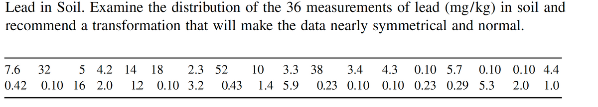

Transcribed Image Text:Lead in Soil. Examine the distribution of the 36 measurements of lead (mg/kg) in soil and
recommend a transformation that will make the data nearly symmetrical and normal.
7.6
0.42
32 5 4.2 14 18 2.3 52 10 3.3 38 3.4 4.3 0.10 5.7 0.10 0.10 4.4
0.10 16 2.0 1.2 0.10 3.2 0.43 1.4 5.9 0.23 0.10 0.10 0.23 0.29 5.3 2.0 1.0
Expert Solution
This question has been solved!
Explore an expertly crafted, step-by-step solution for a thorough understanding of key concepts.

Step by stepSolved in 2 steps

Knowledge Booster

Similar questions
- 1. A researcher is interested in knowing if there is a relationship between the age (years) and height (centimeters) of boys born in the United States in 1990. Age Height (cm) .5 50.8 2 83.8 3 91.4 5 106.6 7 119.3 10 137.1 14 157.5 Using the data in the above table, provide the following information: a. What are your conclusions and observations about the relationship between the two variables b.What is the value of the intercept a c. What is the value of the slope b d. Write the linear regression equationarrow_forward5 and 6. The following data was collected from 1 bag of Hershey Kisses®. Each Kiss® was weighed in grams with the wrapper and recorded in the table below. Hershey claims that there are 368 grams of chocolate in one bag. Hershey Kiss Weights in Grams 4.76 4.72 4.74 4.55 4.91 4.74 4.78 4.71 4.80 4.78 4.78 4.75 4.79 4.82 4.91 4.83 4.68 4.74 4.70 4.80 4.70 4.76 4.70 4.83 4.93 4.74 4.84 4.82 4.76 4.77 4.72 4.78 4.83 4.75 4.74 4.68 4.84 4.71 4.71 4.76 4.66 4.78 4.73 4.74 4.92 4.77 4.80 4.79 4.86 4.64 4.78 4.70 4.75 4.78 4.76 4.83 4.66 4.77 4.83 4.78 4.69 4.81 4.68 4.78 4.88 4.72 4.85 4.85 4.81 4.74 4.80 4.82 4.84 4.70 4.85 4.70 4.81 4.72 4.79 4.73 4.61 Based on Hershey's® claim for 368 total net grams of chocolate in the bag, approximately how many Kisses® too many or too few are there? Assume that the Kisses® were weighed with the wrapper, each wrapper weighs 0.12 grams, and the net grams listed on the bag are for the chocolate only. Give some possible…arrow_forwardThe weights (in pounds) of 6 vehicles and the variability of their braking distances (in feet) when stopping on a dry surface are shown in the table. Can you conclude that there is a significant linear correlation between vehicle weight and variability in braking distance on a dry surface? Use a = 0.05. Weight, x Variability in braking distance, y 5980 5370 6500 5100 5820 4800 1.72 1.97 1.87 1.63 1.64 1.50 Click here to view a table of critical values for Student's t-distribution. Setup the hypothesis for the test. Ho: Ha: P Identify the critical value(s). Select the correct choice below and fill in any answer boxes within your choice. (Round to three decimal places as needed.) O A. The critical value is. B. The critical values are - to and to %3D Calculate the test statistic. t= (Round to three decimal places as needed.) What is your conclusion? There enough evidence at the 5% level of significance to conclude that there a significant linear correlation between vehicle weight and…arrow_forward
- A. run a simple regression- dependent variable is Weeks, independent variable is Age. B. run a multiple regression with dependent variable weeks and independent variable-age, married, head, manager and sales. C. Create the regular and standardized residual plots for both. Please show the tables when entering values of the regression for both the outputs and the scatter plots.arrow_forwardQ. 3 We are given the following data for a city: Population of the city on March 30, 2020 = 183,000 Number of new active cases of TB occurring between January 1 and June 30, 2020 26 Number of active TB cases according to the city register on January 1, 2020 = 264 Find the (i) Cumulative incidence of active cases of TB for the 6-month period3; (ii) Prevalence of active TB as of June 30, 2020.arrow_forward14. The following table gives the miles per gallon and the load capacity for 6 SUV's. Miles per Gallons Load Сарacity 19 860 17 970 16 1035 16 1165 14 1180 13 1360 a. Develop a scatter diagram for the data. b. How would you characterize the relationship between miles per gallon and load capacity?arrow_forward
- Use the given data to find the equation of the regression line. Examine the scatterplot and identify a characteristic of the data that is ignored by the regression line. 11 9 12 8 11 13 4 13 6. 6 У 7.25 7 12.94 7.22 8.15 9.27 6.33 5.3 8.52 6.14 5.46 Create a scatterplot of the data. Choose the correct graph below. O B. OC. O D. O A. Ay 25- Ay 25- 25- 25- 20- 20 20- 20 15 15 15 15 10 10 10- 10 5- 5- 5- 5- 0- 05 10 15 20 25 05 10 15 20 25 0- 05 10 15 20 25 0 5 10 15 20 25 Find the equation of the regression line. (Round the constant two decimal places as needed. Round the coefficient to three decimal places as needed.) Identify a characteristic of the data that is ignored by the regression line. O A. There is no trend in the data. O B. The data has a pattern that is not a straight line. C. There is an influential point that strongly affects the graph of the regression line. D. There is no characteristic of the data that is ignored by the regression line. Click to select your answer(s).…arrow_forwardCan you please check my workarrow_forward1. A study of the relation between the waistline and percent body fat in men yielded the data shown (waistline measurement in inches). waistline (x) 34.7 46.5 32.8 41.3 29.8 39.3 35.7 29.0 percent fat (y) 21.8 33.6 13.4 27.1 13.7 30.2 18.5 11.2 x = 36.1375 y = 21.1875 SSxx = 248.53875 SSay = 332.67375 SSyy = 494.30875 (a) Find the proportion of the variability in percent body fat that is accounted for by the size of the waistline. Explain fully. (b) Find the regression line for predicting y from x. (c) Construct a 95% confidence interval for the average percent body fat of all men whose waistline size is 34.0 inches. (d) test HO: Beta1 is 0 vs. Ha : Beta1 is not 0, compute the appropriate test statistic and p-value, then make your decision at a = 0.05. (e) Construct a 90% confidence interval for beta1. (f) Compute a 90% confidence interval for the average percent fat when waistline is 35.arrow_forward
- 4.) A person's muscle mass is expected to decrease with age. To explore this relationship, a researcher randomly selected 10 persons from ages 40 to 79 years old and measured their muscle mass (unit). The result is as follows: X (age) Y (muscle mass) 71 64 43 67 56 73 68 56 76 65 82 91 100 68 87 73 78 80 65 84 Based on the given data, do the following: a) Plot the scatter diagram of the given data. [3pts] b) Obtain the regression line equation. [4pts] c) Estimate the muscle mass when age of the person is 60 years old. [3pts] 5.) Recognize how each shape has transformed. [2pts each] a.) b.) c.)arrow_forwardFrom the graphs displayed, is there evidence to suggest that there is a positive linear relationship between Square Feet and Bathrooms, for the population of real estate represented by this sample? Be sure to provide numeric support in your answer.arrow_forward5. Explain what the correlation coefficient tells you about the relationship between your variables. 7. Interpret the slope of the regression equation in terms of the variables in your data set.arrow_forward
arrow_back_ios
arrow_forward_ios
Recommended textbooks for you
- MATLAB: An Introduction with ApplicationsStatisticsISBN:9781119256830Author:Amos GilatPublisher:John Wiley & Sons Inc
 Probability and Statistics for Engineering and th...StatisticsISBN:9781305251809Author:Jay L. DevorePublisher:Cengage Learning
 Statistics for The Behavioral Sciences (MindTap C...StatisticsISBN:9781305504912Author:Frederick J Gravetter, Larry B. WallnauPublisher:Cengage Learning
  Elementary Statistics: Picturing the World (7th E...StatisticsISBN:9780134683416Author:Ron Larson, Betsy FarberPublisher:PEARSON
 The Basic Practice of StatisticsStatisticsISBN:9781319042578Author:David S. Moore, William I. Notz, Michael A. FlignerPublisher:W. H. Freeman
 Introduction to the Practice of StatisticsStatisticsISBN:9781319013387Author:David S. Moore, George P. McCabe, Bruce A. CraigPublisher:W. H. Freeman
MATLAB: An Introduction with Applications
Statistics
ISBN:9781119256830
Author:Amos Gilat
Publisher:John Wiley & Sons Inc
Probability and Statistics for Engineering and th...
Statistics
ISBN:9781305251809
Author:Jay L. Devore
Publisher:Cengage Learning
Statistics for The Behavioral Sciences (MindTap C...
Statistics
ISBN:9781305504912
Author:Frederick J Gravetter, Larry B. Wallnau
Publisher:Cengage Learning
Elementary Statistics: Picturing the World (7th E...
Statistics
ISBN:9780134683416
Author:Ron Larson, Betsy Farber
Publisher:PEARSON
The Basic Practice of Statistics
Statistics
ISBN:9781319042578
Author:David S. Moore, William I. Notz, Michael A. Fligner
Publisher:W. H. Freeman
Introduction to the Practice of Statistics
Statistics
ISBN:9781319013387
Author:David S. Moore, George P. McCabe, Bruce A. Craig
Publisher:W. H. Freeman