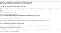
John Hopkins University (JHU) reports Covid-19 statistics daily for every US state and many countries in the world. In this problem we are concerned with four of them for some region, say Arizona. Each one is a function of time t, in days. P(t) - Cumulative Confirmed Cases: total number of cases confirmed before day t N(t) - Daily New Cases: number of cases first confirmed on day t R(t) - Cumulative Recovered or Removed: total number of people who were confirmed to have Covid-19 but have recovered or who have passed before day t Many communities are interested in A(t) A(t), the number of people infected on day t-1 t-1. This is important because it gives the community an idea of the hospital capacity they may need. a.) What is the meaning of P(t+1)? Answer in words. b.) How are P(t+1) and P(t) and N(t) related? Write an equation connecting these three quantities and explain why this is true c.) What is the meaning of N(t-1) and N(t-2)? Answer in words. d.) How can you find A(t) from P(t) and one of the other two functions, N and R? Use this to write a formula for A(t). (For this problem, assume no one is infectious the day they get diagnosed.) Then explain e.) Use the fact that most Covid cases last for two weeks (14 days) and assume that people are infectious for the whole 14 days. Write a formula for A(t) in terms of the function N (and no other functions).

interpret the domain nad range and increase / decrease of theb graph in terms of the problem situation

In a study a group of 50 adults were asked how comfortable they felt around 5 types of animals: dogs, cats, cows, horses and sheep. For each type of animal, each respondent gave a number between 0 and 100 to indicate their comfort level (0 being 'hate being around' to 100 being 'love being around'). The data are given in Table 10, along with the loadings of the first two principal components. Variable (b) (c) X₁ X₂ X3 X4 X5 Animal Mean Dogs 74.5 Cats 76.2 Cows 45.2 Horses 51.2 Sheep 48.3 Table 10 Standard Deviation Component 1 Loadings 8.1 7.5 7.1 8.6 6.9 0.724 -0.684 0.080 -0.040 -0.017 Component 2 0.387 0.425 0.464 0.449 0.503 (a) The data were not standardized prior to being analyzed using principal components. Give 2 reasons why the decision not to standardize is reasonable for these data. Interpret each of the 2 components. Justify your answer. Suppose a decision was taken to standardize the data after all. Calculate the values of the standardized variables for a person whose…

31. Table 4.3 shows the population of Pennsylvania in each 10-year census between 1830 and 1950. Table 4.3 Population of Pennsylvania Population in Years since 1820 thousands 10 1348 20 1724 30 2312 40 2906 50 3522 60 4283 70 5258 80 6302 90 7665 100 8720 10 9631 120 9900 130 10,498 Source: Bureau of the Census, uS. Chamber of Cammerce. (a) Find the logistic regression for the data. (b) Graph the data in a scatter plot and superimpose the regres- sion curve. (c) Use the regression equation to predict the Pennsylvania popu- lation in the 2000 census. (d) In what year was the Pennsylvania population growing the fastest? What significant behavior does the graph of the regres- sion equation exhibit at that point? (e) What does the regression equation indicate about the popula- tion of Pennsylvania in the long run?

If another variable systematically co-varies with the independent variable, then we likely have an extraneous variable b. a dependent variable an ex post facto design a confounding variable

Q8. Are rent rates influenced by the student population in a college town? Let rent be the average monthly rent paid on rental units in a college town in the United States. Let pop denote the total city population, avginc the average city income, and pctstu the student population as a percentage of the total population. One model to test for a relationship is log(rent) = 0.03048 + 0.5 * log(pop) +0.673 log(avginc) + 0.0046 pctstu (.844) (.039) (.081) (.0028) i) State the null hypothesis that the percentage of students relative to the population has no ceteris paribus effect on monthly rents. State the alternative that there is an effect. What signs do you expect for B₁ and ₂ ? The equation estimated for 64 college towns is log(rent) = 0.03048 + 0.5 * log(pop) + 0.673 log(avginc) + 0.0045 pctstu (.844) (.039) (.081) (.0017) Standard errors are given in the parentheses. test the null hypothesis H_0 that "10% ceteris paribus increase in population is associated with about a 6.6% increase…

A doctor notes the variables listed in the following table from every patient before admitting in his hospital.  Which of the following variables are qualitative and which are quantitative?  Which qualitative variables are nominal or ordinal? Which quantitative variables are discrete or continuous?   ( 1 )  Gender (Male or Female)   ( 2 ) Weight (lbs)   ( 3 ) Phone Number   ( 4 ) Height (cm)   ( 5 ) Marital Status (Single, Married, Divorce, Widow)   ( 6 ) Systolic Blood Pressure (mm of pressure)   ( 7 ) Temperature (degree F)   ( 8 ) Level of Calcium (microgram/milimeter)   ( 9 ) Family of Income ( Amount)   ( 10 ) Wihte Blood Cells

Which of these statements is not a condition for an exposure to quality as a risk factor?   There is a dose-response relationship   There is temporality of the exposure and the disease in terms of occurrence   The observed relationship between exposure and the disease in not due to some source of error in the design   The observed relationship between exposure and the disease is due to due to some source of error in the design.

A researcher wants to determine if the exam scores of the students are dependent on the length of time spent in studying the subject. Ten students in a certain class were taken and the results are shown in the table below where X is the time spent in studying the subject in hours and Y is the examination scores. X (time) Y (score) 1.5 80 3.0 83 1.25 83 0.5 70 3.5 85 2.5 75 1.0 70 3.0 90 2.5 86 4.0 91 Determine the simple linear regression equation Y = a + bX. (round off values up to 1 decimal place)

I have collected real data on the sale of a microwavable cup of soup across 20 different cities for the same time period (a month).  The variables in the dataset are:   Quantity sold in the city for that month:  Measured in thousands of units Price:  measured in dollars Average Income in the city:  Measured in thousands of dollars Ads:  Average number of ads run in stores for that city during that month. Price of a substitute product:  measured in dollars Population of the city:  measured in thousands of people   The dataset is on Canvas and, using Excel or any other statistical software, please answer the following questions:   1. Describe the patterns in quantity sold and own and rival prices during this time period using basic descriptive statistics.  Graphs are welcome as well.   2. Take the logs of the variables, and estimate the demand function. a. Interpret the R-square. b. Interpret the coefficients for logP and logPsub c. Interpret the p-values associated with each independent…