
MATLAB: An Introduction with Applications
6th Edition
ISBN: 9781119256830
Author: Amos Gilat
Publisher: John Wiley & Sons Inc
expand_more
expand_more
format_list_bulleted
Related questions
Topic Video
Question
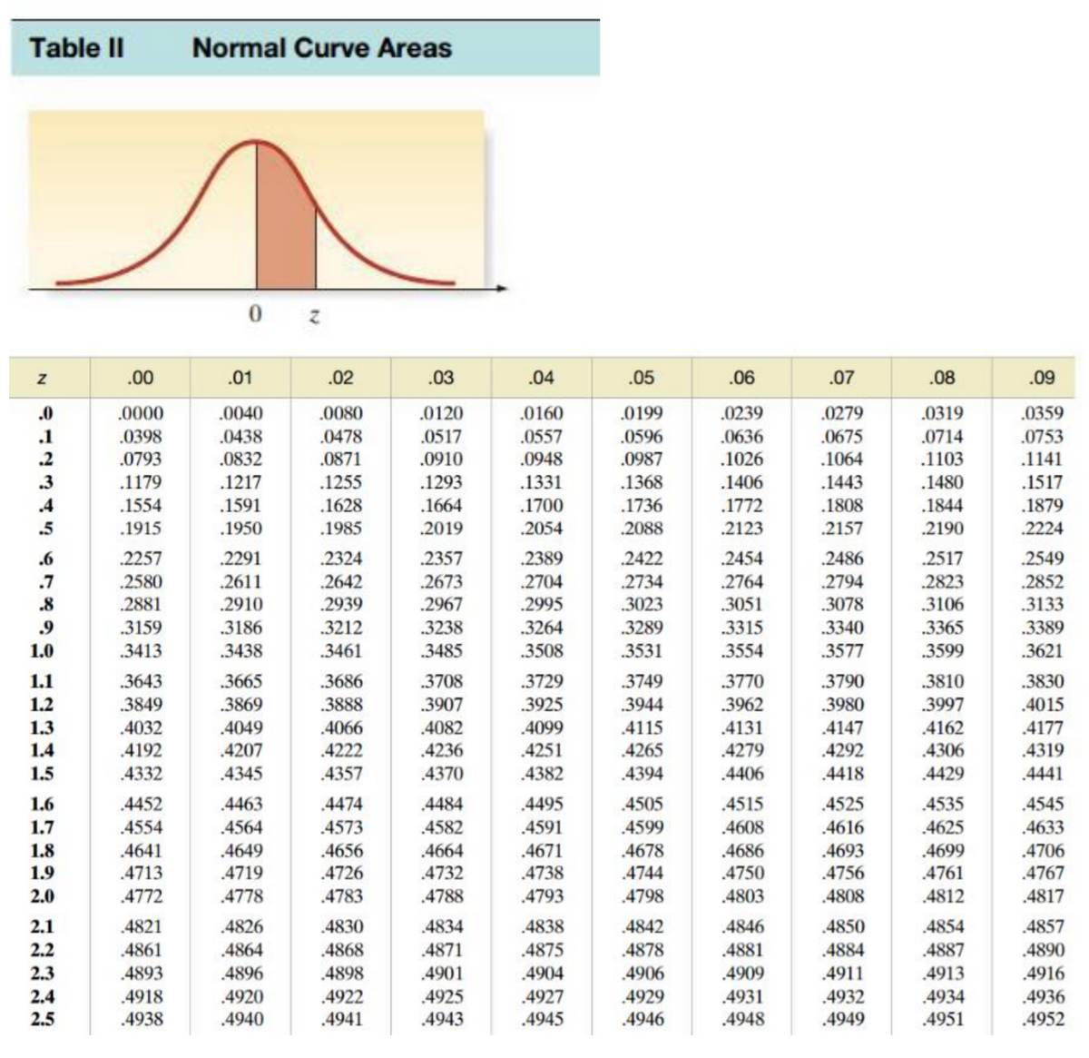

Transcribed Image Text:Table II
Normal Curve Areas
.00
.01
.02
.03
.04
.05
.06
.07
.08
.09
.0
.0000
.0040
.0080
.0120
.0160
.0199
.0239
.0279
.0319
.0359
.0478
.0871
.0596
.0987
.0438
.0517
.0910
.1293
.0675
.1064
.0714
.1103
.1480
.1
.0398
.0557
.0636
.0753
.2
.0793
.0832
.0948
.1026
.1141
.3
.1179
.1217
.1255
.1331
.1368
.1406
.1443
.1517
.1844
.2190
.4
.1554
.1591
.1628
.1664
.1700
.1736
.1772
.1808
.1879
.5
.1915
.1950
.1985
.2019
.2054
.2088
.2123
.2157
.2224
.6
.2257
.2291
.2324
.2357
.2389
.2422
.2454
.2486
.2517
.2549
.2794
.3078
.2580
.2673
.2967
.7
.2611
.2642
.2704
.2734
.2764
.2823
.2852
.3051
.3315
.8
.2881
.2910
.2939
.2995
3023
.3106
.3133
.3340
.3577
.3264
3289
.3365
.3599
.9
.3159
.3186
.3212
.3238
.3389
1.0
.3413
.3438
.3461
.3485
.3508
.3531
.3554
.3621
1.1
.3643
.3665
.3686
.3708
.3729
.3749
.3770
.3790
.3810
.3830
.3849
.4032
.4192
1.2
.3869
.3888
.3907
3925
.3944
.3962
.3980
.3997
.4015
4162
.4306
1.3
.4049
.4066
.4082
.4099
.4115
.4131
.4147
.4177
.4222
.4357
1.4
.4207
.4236
.4251
.4265
.4279
.4292
.4319
1.5
4332
.4345
.4370
.4382
.4394
.4406
4418
4429
.4441
1.6
.4452
.4463
.4474
.4484
.4495
.4505
.4515
4525
4535
.4545
1.7
.4554
.4564
.4573
.4582
.4591
.4599
.4608
.4616
.4625
.4633
.4678
.4744
1.8
.4641
.4671
.4738
.4649
.4656
.4664
.4686
.4693
.4699
.4706
1.9
.4713
.4719
.4726
.4732
.4750
.4756
4761
.4767
2.0
.4772
.4778
.4783
.4788
.4793
4798
.4803
.4808
.4812
.4817
2.1
.4821
.4826
.4830
.4834
.4838
.4842
.4846
.4850
.4854
.4857
.4864
.4896
2.2
.4861
.4868
4871
.4875
.4878
.4881
.4884
.4887
.4890
.4904
.4927
2.3
.4893
.4898
.4901
.4906
.4909
.4911
.4913
.4916
.4925
.4943
.4932
.4949
2.4
.4918
.4920
.4922
4929
.4931
.4934
.4936
2.5
.4938
.4940
.4941
.4945
.4946
.4948
.4951
.4952

Transcribed Image Text:It has been estimated that the 1991 G-car obtains a mean of 35 miles per gallon on the
highway, and the company that manufactures the car claims that it exceeds the estimate in
highway driving. To support its assertion, the company randomly selects 49 1991 G-cars and
records the mileage obtained for each car over a driving course similar to that used to obtain the
estimate. The following data resulted: x = 36.5 miles per gallon, s = 7 miles per gallon.
%3D
a. Find the observed significance level for testing Ho: u= 35 vs. Ha: u> 35.
%3D
b. For what value of significance level a, you will reject the null hypothesis.
Expert Solution
This question has been solved!
Explore an expertly crafted, step-by-step solution for a thorough understanding of key concepts.

This is a popular solution

Trending nowThis is a popular solution!

Step by stepSolved in 4 steps

Knowledge Booster


Learn more about
Need a deep-dive on the concept behind this application? Look no further. Learn more about this topic, statistics and related others by exploring similar questions and additional content below.Similar questions
- Perform PCA or principle component analysis on the following data: х1 x2 x3 810.6 13.4 42.93 1775 24.2 32.319 430.4 5.7 60.434 459.8 9 21.398 802.4 13.9 55.778 279.6 20.4 53.236 288.4 4.6 63.208 152.7 7.3 59.727 253.4 9.9 48.037 358.6 13.5 48.288 72 12.8 36.507 205 5.9 37.195 253.6 15.8 36.964 416.5 12.3 42.83 1075.9 17.1 39.684 Answer the following questions based on the PCA: • How many principle components were created? • What percent of total variance is accounted for by the calculated principal components? (Round to 2 decimal places) • What are the weights for computing the first principle component scores? (Round to 4 decimal places) o x1: • x2: o x3:arrow_forwardA botanist grew 24 pepper plants on the same greenhouse bench. After 21 days, she measured the total stem length (cm) of each plant, and obtained the following values: 9.8 12.1 13.1 Min Q1 10.1 12.2 13.2 Match the values with each statistic given below: Median Q3 Max 10.9 12.2 13.2 11.3 12.3 13.4 11.8 12.5 13.5 A. 12.40 B. 9.8 C. 12.38 D. 11.97 E. 14.10 F. 11.90 G. 13.35 H. 12.39 1. 12.35 J. 13.20 K. 11.95 L. 12.22 11.9 12.6 13.5 12.0 12.7 13.6 12.0 13.0 14.1arrow_forwardThe accompanying data file contains 10 observations with two variables, x1 and x2. picture Click here for the Excel Data File x1 x26.63 0.854.89 0.1911.24 1.4723.98 0.743.89 2.3633.99 0.804.56 1.6410.42 0.906.78 1.1117.32 0.99 a-1. Using the original values, compute the Euclidean distance for all possible pairs of the first three observations. (Round intermediate calculations to at least 4 decimal places and your final answers to 2 decimal places.) a-2. Using the z-score standardized values, compute the Euclidean distance for all possible pairs of the first three observations. (Round intermediate calculations to at least 4 decimal places and your final answers to 2 decimal places.) b-1. Using the original values, compute the Manhattan distance for all possible pairs of the first three observations. (Round intermediate calculations to at least 4 decimal places and your final answers to 2 decimal places.) b-2. Using the the z-score…arrow_forward
- Joan's Nursery specializes in custom-designed landscaping for residential areas. The estimated labor cost associated with a particular landscaping proposal is based on the number of plantings of trees, shrubs, and so on to be used for the project. For cost-estimating purposes, managers use two hours of labor time for the plant- ing of a medium-sized tree. Actual times from a sample of 10 plantings during the past month follow (times in hours).2.1 2.2 1.7 1.6 2.3 3.1 1.5 2.6 2.4 2.2 With a .05 level of significance, test to see whether the mean tree-planting time differs from two hours. a. State the null and alternative hypotheses. b. Compute the sample mean. c. Compute the sample standard deviation. d. What is the p-value? e. What is your conclusion?arrow_forwardBecause the mean is very sensitive to extreme values, it is not a resistant measure of center. By deleting some low values and high values, the trimmed mean is more resistant. To find the 10% trimmed mean for a data set, first arrange the data in order, then delete the bottom 10% of the values and delete the top 10% of the values, then calculate the mean of the remaining values. Use the axial loads (pounds) of aluminum cans listed below for cans that are 0.0111 in. thick. Identify any outliers, then compare the median, mean, 10% trimmed mean, and 20% trimmed mean. 246 259 268 274 275 278 280 283 285 285 286 288 289 292 294 294 296 299 309 506 Identify any outliers. Select the correct choice below and, if necessary, fill in the answer box to complete your choice. OA. The outlier(s) is/are pounds. (Type a whole number. Use a comma to separate answers as needed.) B. There are no outliers.arrow_forwardhe level of cretaine phosphokinase (CPK) in blood samples measures the amount of muscle damage for athletes. At Jock State University, the level of CPK was determined for each of 25 football players and 15 soccer players before and after practice. The two groups of athletes are trained independently. The data summary is as follows : For football players: Data for Football players n=25 Before Practice After Practice Difference (Before-After) Mean 254.73 225.6 29.13 Standard deviation 115.5 132.6 21.00 For soccer players: Data for Soccer players n=15 Before Practice After Practice Difference (Before-After) Mean 177.1 173.8 3.3 Standard deviation 60.7 64.4 6.88 Assume that all the data above are normal Test the claim that the mean CPK level has DECREASED for soccer players AFTER exercise (compared to the mean BEFORE exercise), using α=0.10. AFTER practice, do football players have a DIFFERENT mean CPK values compared to soccer players? Test this claim by…arrow_forward
- Determine whether the given value is from a discrete or continuous data set. An impact SUV has a gas tank that can hold 15.21 gal.arrow_forwardThe following relative frequency histogram presents the weights (in lb) of a sample of visitors to a health clinic. What percent of visitors to the health clinic weighed less than 150 lb?arrow_forwardGiven the weekly price and quantity (Qx and (Px) data for Andy’s ice cream over the past 12 weeks and the price of another ice-cream flavor (Po) as: Qx 84 82 85 83 82 84 87 81 82 79 82 78 Px 8.50 9.00 8.75 9.25 9.50 9.25 8.25 10.00 10.00 10.50 9.50 10.25 Po 5.25 6.00 6.00 6.50 6.25 6.25 5.25 7.00 7.25 7.25 6.75 7.25 a. Use excel regression to estimate the weekly demand for Andy’s ice-cream (attach the output of the regression estimate (Hint: Use regression in excel to find the estimated demand function: Enter the data in excel, click on Data Analysis, and use the regression command). b. Are the coefficients on the two prices statistically significantly different from zero at the 5% significance level? How do you know? c. What the R2? d. Explain what R2 means.arrow_forward
- (3-B is needed to answer it I am only asking for question 4.) 3) You go out and collect the following estimates of earthworms / acre:54,276 57,378 51,108 66,190 66,232 59,018 57,159These data yield the following: ̄y = 59,765.86, and s = 5,689.606a) Construct a 90% CI for these data.b) Construct a 99% CI for these data.c) Darwin once estimated that an acre of soil had about 50,000 worms in it. Is his estimateconsistent with the data above? (Historical note: His estimate was considered way too high inhis day). 4) Consider the results of 3(b). Notice that all the data fit within the 99% confidence interval. Is thisusually the case (in other words, will a 99% CI contain most of the observations)?Caution: a lot of people get this wrong! Here's a hint: suppose you had measured the worms in6000 acres (instead of just 7). What happens to the confidence interval? If you're not sure,substitute 6,000 for 7 in your calculation for (b) to see what happens.arrow_forwardListed below are the measured radiation absorption rates ( in 5 - number summary . W/kg) corresponding to 11 cell phones . Use the given data to construct a boxplot and identify the 1.49,1.25, 1.38, 1.04, 1.46, 1.31, 1.28, 0.73, 1.41, 0.58, 1.36arrow_forwardIn the accompanying data table, the entries are for five different years and consist of the weights (metric tons) of lemons imported from another country and car crash fatality rates per 100,000 population. The data are based on data from a scientific publication. Lemon Imports: 220 274 355 478 539 Crash Fatality Rate: 16.7 14.8 15.2 14.7 15.8 Given that the data are matched and considering the units of the data, does it make sense to use the difference between each pair of values? Why or why not? Choose the correct answer below. A. No, it does not make sense to use the difference between each amount of lemon imports and car crash fatality rate in the same column,because the terms should be added. B. Yes, it does make sense to use the difference between each amount of lemon imports and car crash fatality rate in the same column, because they are measurements obtained from the same year. C. No, it does not make…arrow_forward
arrow_back_ios
SEE MORE QUESTIONS
arrow_forward_ios
Recommended textbooks for you
- MATLAB: An Introduction with ApplicationsStatisticsISBN:9781119256830Author:Amos GilatPublisher:John Wiley & Sons Inc
 Probability and Statistics for Engineering and th...StatisticsISBN:9781305251809Author:Jay L. DevorePublisher:Cengage Learning
 Statistics for The Behavioral Sciences (MindTap C...StatisticsISBN:9781305504912Author:Frederick J Gravetter, Larry B. WallnauPublisher:Cengage Learning
  Elementary Statistics: Picturing the World (7th E...StatisticsISBN:9780134683416Author:Ron Larson, Betsy FarberPublisher:PEARSON
 The Basic Practice of StatisticsStatisticsISBN:9781319042578Author:David S. Moore, William I. Notz, Michael A. FlignerPublisher:W. H. Freeman
 Introduction to the Practice of StatisticsStatisticsISBN:9781319013387Author:David S. Moore, George P. McCabe, Bruce A. CraigPublisher:W. H. Freeman
MATLAB: An Introduction with Applications
Statistics
ISBN:9781119256830
Author:Amos Gilat
Publisher:John Wiley & Sons Inc
Probability and Statistics for Engineering and th...
Statistics
ISBN:9781305251809
Author:Jay L. Devore
Publisher:Cengage Learning
Statistics for The Behavioral Sciences (MindTap C...
Statistics
ISBN:9781305504912
Author:Frederick J Gravetter, Larry B. Wallnau
Publisher:Cengage Learning
Elementary Statistics: Picturing the World (7th E...
Statistics
ISBN:9780134683416
Author:Ron Larson, Betsy Farber
Publisher:PEARSON
The Basic Practice of Statistics
Statistics
ISBN:9781319042578
Author:David S. Moore, William I. Notz, Michael A. Fligner
Publisher:W. H. Freeman
Introduction to the Practice of Statistics
Statistics
ISBN:9781319013387
Author:David S. Moore, George P. McCabe, Bruce A. Craig
Publisher:W. H. Freeman