Is it defense or offense that wins football games? The accompanying data file includes a team’s winning record (Win in %), the average number of yards gained, and the average number of yards allowed during a recent NFL season.
| Team | Win | Yards_Gained | Yards_Allowed |
| Arizona Cardinals | 46.9 | 366.8 | 305.2 |
| Atlanta Falcons | 68.8 | 415.8 | 371.2 |
| Baltimore Ravens | 50.0 | 347.7 | 322.1 |
| Buffalo Bills | 43.8 | 354.1 | 357.0 |
| Carolina Panthers | 37.5 | 343.7 | 359.8 |
| Chicago Bears | 18.8 | 356.5 | 346.8 |
| Cincinnati Bengals | 40.6 | 356.9 | 350.8 |
| Cleveland Browns | 6.2 | 311.0 | 392.4 |
| Dallas Cowboys | 81.2 | 376.7 | 343.9 |
| Denver Broncos | 56.2 | 323.1 | 316.1 |
| Detroit Lions | 56.2 | 338.8 | 354.8 |
| Green Bay Packers | 62.5 | 368.8 | 363.9 |
| Houston Texans | 56.2 | 314.7 | 301.3 |
| Indianapolis Colts | 50.0 | 364.4 | 382.9 |
| Jacksonville Jaguars | 18.8 | 334.9 | 321.7 |
| Kansas City Chiefs | 75.0 | 343.0 | 368.5 |
| Miami Dolphins | 25.0 | 262.7 | 337.0 |
| Minnesota Vikings | 62.5 | 332.8 | 382.6 |
| New England Patriots | 50.0 | 315.1 | 314.9 |
| New Orleans Saints | 87.5 | 386.2 | 326.4 |
| New York Giants | 43.8 | 426.0 | 375.4 |
| New York Jets | 68.8 | 330.7 | 339.7 |
| Oakland Raiders | 31.2 | 329.2 | 342.4 |
| Philadelphia Eagles | 75.0 | 373.3 | 375.1 |
| Pittsburgh Steelers | 43.8 | 337.4 | 342.8 |
| Saint Louis Rams | 68.8 | 372.6 | 342.6 |
| San Diego Chargers | 31.2 | 356.8 | 347.1 |
| San Francisco 49ers | 12.5 | 308.1 | 406.4 |
| Seattle Seahawks | 65.6 | 357.2 | 318.7 |
| Tampa Bay Buccaneers | 56.2 | 346.4 | 367.9 |
| Tennessee Titans | 56.2 | 358.0 | 357.5 |
| Washington Redskins | 53.1 | 403.4 | 377.9 |
1. Compare two simple linear regression models where Model 1 predicts Win as a
Note: Negative values should be indicated by a minus sign. Round your answers to 2 decimal places.
2. Estimate a linear regression for Model 3, that applies both Yards Gained and Yards Allowed to forecast Win.
Note: Negative values should be indicated by a minus sign. Round your answers to 2 decimal places.
3. Which of the models is a better predictor to forecast a win?
1.
Model 1 predicts Win as a function of Yards Gained:
Excel Procedure:
- Enter Win and Yards Gained data in Excel
- Data>Data Analysis> ‘Regression’
- Select Wins under ‘Input Y Range’
- Select Yards Gained under ‘Input X Range’
- Click on ‘OK’.
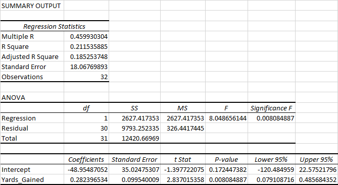
Output:

Regression Equation:
wins=-48.95+0.28Yards_Gained
From the output, the R^2 value is 0.2115.
Trending nowThis is a popular solution!
Step by stepSolved in 4 steps with 3 images

- Explain HOUSING STATISTICS?arrow_forwardCalculate the difference between List Price and Sale Price for each condominium by creating a new column and use the Data Analysis Toolpak Descriptive Statistics for that new column for Gulf View. Gulf View Condominiums List Price Sale Price Days to Sell 478.0 474.0 133 394.0 329.0 85 537.0 532.0 82 542.5 543.5 91 353.9 314.9 132 553.0 506.0 74 143.9 168.0 197 201.0 224.0 59 962.0 919.0 91 317.0 324.0 117 328.0 291.0 95 883.0 823.0 277 965.0 1012.0 103 470.0 421.0 61 298.0 290.0 43 362.0 361.0 47 319.0 301.0 93 524.0 469.0 159 434.0 370.0 158 683.0 680.0 153 409.0 405.0 18 681.0 656.0 6 321.0 314.0 140 412.0 393.0 89 366.0 344.0 105 474.0 493.0 43 906.0 871.0 125 444.0 468.0 170 415.0 426.0 212 259.0 225.0 99 647.0 633.0 85 611.0 594.0 90 352.0 321.0 98 596.0 579.0 34 319.0 288.0 139 190.0 219.0 53 379.0 394.0 148 450.0 429.0 49 488.0 455.0 85 443.0 423.5 156arrow_forwardThis table shows the age distribution of people in the United States in 2010. a. Complete the last column of a copy of this table. Proportion of Population! Age Number of People Under 18 74,181,467 0.2403 18-44 112,806,642 45-64 81,489,445 0.2639 65 and Over 40,267,984 Total 308,745,538 Source: Age and Sex Composition: 2010, Census Briefs, www.census.gov/prod/ cen2010/briefs/c2010br-03.pdf The fellew USarrow_forward
- Given the following data set: $1.42, $1.27, $1.28, $1.48, $1.36, $1.44, $1.46, $1.32, $1.33, $1.33 $1.23, $1.38, $1.43, $1.28, $1.43, $1.49, $1.37, $1.26, $1.26, $1.38 Determine the frequencies of gasoline prices for each given class. Frequency Relative Frequency Class < $1.25 $1.25 < $1.30 $1.30 $1.35 $1.35 $1.40 $1.40 < $1.45 $1.45 CHECK ANSWERarrow_forwardgiven data: 2.1, 2.8, 3.7, 4.1, 4.6, 5.8, 6.3, 7.4, 8.2, 8.5, 9.6, 10.1, 10.3, 10.9, 11.0, 11.8, 12.4, 13.6, 13.9, 14.3, 14.6, 15.5, 15.9, 16.7, 16.9 Can I get help with... 6a) Two data sets both have a mean of 50. One has a standard deviation of 2 and the other has a standard deviation of 10. Describe what is different about these two data sets. b) Since the mean and the median both describe the same characteristic, explain why they are not always the same. (no formulas) c) When and why would the mean be better to use than the median?arrow_forwardUse this dataset for your analysis software.Cost-to-charge ratio (the percentage of the amount billed that represents the actual cost) for inpatient and outpatient services at 11 Oregon hospitals is shown in the following table. A scatterplot of the data is also shown. Cost-to-Charge Ratio Hospital OutpatientCare InpatientCare 1 62 80 2 66 76 3 63 75 4 51 62 5 75 100 6 65 88 7 56 64 8 45 50 9 48 54 10 71 83 11 54 100 The least-squares regression line with y = inpatient cost-to-charge ratio and x = outpatient cost-to-charge ratio is = -1.1 + 1.29 x. (a) Is the observation for Hospital 11 an influential observation? Yes or No (b) Is the observation for Hospital 11 an outlier? Yes or No (c) Is the observation for Hospital 5 an influential observation? Yes or No (d) Is the observation for Hospital 5 an outlier? Yes or Noarrow_forward
- The average number of minutes Americans commute to work is 27.7 minutes (Sterling's Best Places, April 13, 2012). The average commute time in minutes for 48 cities are as follows: Click on the datafile logo to reference the data. DATA file Albuquerque Atlanta Austin Baltimore Boston Charlotte Chicago Cincinnati Cleveland Columbus Dallas Denver Detroit El Paso Fresno Indianapolis 23.3 28.3 24.6 32.1 31.7 25.8 38.1 24.9 26.8 23.4 28.5 28.1 29.3 24.4 23.0 24.8 Jacksonville Kansas City Las Vegas Little Rock Los Angeles Louisville Memphis Miami Milwaukee Minneapolis Nashville New Orleans New York Oklahoma City Orlando Philadelphia 26.2 Phoenix 23.4 Pittsburgh Portland 28.4 20.1 32.2 21.4 23.8 30.7 24.8 23.6 25.3 31.7 43.8 22.0 27.1 34.2 Providence Richmond c. What is the mode for these 48 cities? Select your answer - Sacramento Salt Lake City San Antonio San Diego San Francisco San Jose Seattle St. Louis Tucson Tulsa Washington, D.C. 28.3 25.0 26.4 23.6 23.4 25.8 20.2 26.1 24.8 32.6 28.5…arrow_forwardUse the coefficient of variation to determine whether coffee prices or gasoline prices were more stable in 2015. Use the population standard and population mean of each set of data. What is the coefficient of variation for the price of a pound of coffee and a pound of gasoline?arrow_forwardGasoline tax. find the mean, median, and mode for the data in the following table. (source: American Petroleum Institute.) State Gasoline Tax, 2017 STATE TAX(CENTS PER GAL.) winsconsin 32.9 new york 43.9 connecticut 39.9 nebraska 28.2 kansas 24.0 texas 20.0 california 38.1 tennessee 21.4arrow_forward
- A report gave the accompanying data for the 50 U.S. states on the percentage of the population that was born in the state and is still living there. The data values have been arranged in order from largest to smallest. 75.6 71.4 69.6 69.0 68.6 67.5 66.7 66.3 66.1 66.0 66.0 65.2 64.6 64.3 63.8 63.7 62.8 62.6 61.8 61.8 61.5 61.1 59.2 59.0 58.7 57.3 57.1 55.8 55.8 55.5 55.3 54.9 54.7 54.5 54.0 54.0 53.6 53.5 52.8 52.5 50.2 50.2 48.9 48.7 48.2 47.3 43.4 40.4 35.8 28.2 (a) Find the values of the median, the lower quartile, and the upper quartile. (Enter your answers to one decimal place.) median = lower quartile = upper quartile = (b) The two smallest values in the data set are 35.8 (Alaska) and 28.2 (Wyoming). Are these two states outliers? Alaska is an outlier, but Wyoming is not.Neither Alaska nor Wyoming are outliers. Wyoming is an outlier, but Alaska is not.Alaska and Wyoming are both outliers. (c) Construct a boxplot for this data set.arrow_forwardEach year forbes ranks the world’s most valuable brands. A portion of the data for 82 ofthe brands in the 2013 forbes list is shown in Table 2.12 (forbes website, february, 2014).The data set includes the following variables:brand: The name of the brand.Industry: The type of industry associated with the brand, labeled Automotive& Luxury, Consumer Packaged Goods, financial Services, Other, Technology.brand Value ($ billions): A measure of the brand’s value in billions of dollarsdeveloped by forbes based on a variety of financial information about the brand.1-Yr Value Change (%): The percentage change in the value of the brand over theprevious year.brand Revenue ($ billions): The total revenue in billions of dollars for the brand.a. Prepare a crosstabulation of the data on Industry (rows) and brand Value ($ billions).Use classes of 0–10, 10–20, 20–30, 30–40, 40–50, and 50–60 for brand Value($ billions).b. Prepare a frequency distribution for the data on Industry.arrow_forwardIdentify the type of observational study (cross-sectional, retrospective, or prospective) described below. A research company uses a device to record the viewing habits of about 5000 households, and the data collected over the next 6 years will be used to determine whether the proportion of households tuned to a particular news program decreases. Which type of observational study is described in the problem statement? A retrospective study A prospective study A cross-sectional studyarrow_forward
 A First Course in Probability (10th Edition)ProbabilityISBN:9780134753119Author:Sheldon RossPublisher:PEARSON

