
MATLAB: An Introduction with Applications
6th Edition
ISBN: 9781119256830
Author: Amos Gilat
Publisher: John Wiley & Sons Inc
expand_more
expand_more
format_list_bulleted
Related questions
Question
- ) In estimating the regression in problem #2, you are also concerned that the t-statistics may be inflated because of the presence of conditional heteroscedasticity. There are 214 observations and 3 independent variables.
You conduct a regression of the squared residuals against the dummy variables X1, X2, and X3 and find that for the squared residuals regression:
|
|
Multiple R |
0.4145 |
|
|
R Square |
0.1718 |
|
|
Adjusted R Square |
0.1600 |
|
|
SEE |
92.3760 |
- Conduct a Breusch–Pagan test at the 0.05 level to see if conditional heteroskedasticity is present and from your results, what needs to be done?
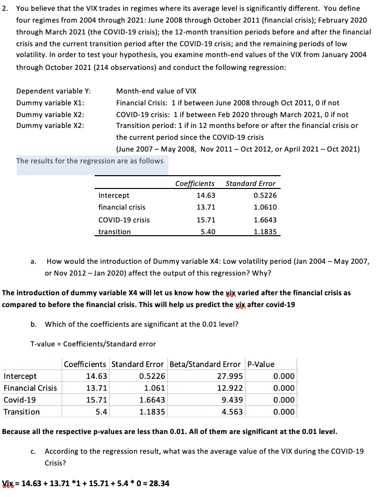

Transcribed Image Text:2. You believe that the VIX trades in regimes where its average level is significantly different. You define
four regimes from 2004 through 2021: June 2008 through October 2011 (financial crisis); February 2020
through March 2021 (the COVID-19 crisis); the 12-month transition periods before and after the financial
crisis and the current transition period after the COVID-19 crisis; and the remaining periods of low
volatility. In order to test your hypothesis, you examine month-end values of the VIX from January 2004
through October 2021 (214 observations) and conduct the following regression:
Dependent variable Y:
Month-end value of VIX
Dummy variable X1:
Financial Crisis: 1 if between June 2008 through Oct 2011, 0 if not
COVID-19 crisis: 1 if between Feb 2020 through March 2021, 0 if not
Transition period: 1 if in 12 months before or after the financial crisis or
Dummy variable X2:
Dummy variable X2:
the current period since the COVID-19 crisis
(June 2007 – May 2008, Nov 2011 – Oct 2012, or April 2021- Oct 2021)
The results for the regression are as follows
Coefficients
Standard Error
Intercept
14.63
0.5226
financial crisis
13.71
1.0610
COVID-19 crisis
15.71
1.6643
transition
5.40
1.1835
а.
How would the introduction of Dummy variable X4: Low volatility period (Jan 2004 – May 2007,
or Nov 2012 - Jan 2020) affect the output of this regression? Why?
The introduction of dummy variable X4 will let us know how the vix varied after the financial crisis as
compared to before the financial crisis. This will help us predict the yix after covid-19
b.
Which of the coefficients are significant at the 0.01 level?
T-value = Coefficients/Standard error
Coefficients Standard Error Beta/Standard Error P-Value
Intercept
14.63
0.5226
27.995
0.000
Financial Crisis
13.71
1.061
12.922
0.000
Covid-19
15.71
1.6643
9.439
0.000
Transition
5.4
1.1835
4.563
0.000
Because all the respective p-values are less than 0.01. All of them are significant at the 0.01 level.
C.
According to the regression result, what was the average value of the VIX during the COVID-19
Crisis?
Vix = 14.63 + 13.71 *1+ 15.71 + 5.4 * 0 = 28.34
Expert Solution
This question has been solved!
Explore an expertly crafted, step-by-step solution for a thorough understanding of key concepts.

Step by stepSolved in 4 steps

Knowledge Booster

Similar questions
- A researcher is investigating possible explanations for deaths in traffic accidents. He examined data from 2000 for each of the 52 cities randomly selected in the US. The data included information on the followingvariables: Deaths: The number of deaths in traffic accidents per city and Income: The median income per cityAs part of his study, he ran the following simple linear regression model as pictured : Question: Based on the above results, the researcher tested the hypotheses ( Null: B1=0 versus Alternative: B1 not equal to 0) using T test. What do we know about the test statistic of the test, what is the approximate p-value, and value of Rsquared? And based on your result, what is your conclusion? Show your work for full credit.arrow_forwardWhere we observe multicollinearity in a multiple regression analysis, two of our independent variables, x-1 and x-4, are so highly correlated they’re almost indistinguishable with respect to their relationship with our dependent (y) variable. Why is that a problem?arrow_forwardSuppose you are to estimate a simple regression for the following population model: Y=B₁ + B₁X + µl From a population of over thousands of observations, a small number of samples were randomly selected. The following is some of the information from the randomly selected sample.arrow_forward
- Parts b, c, and d only please.arrow_forward7. Find slop of a linear regression model for the following data: x = [1, 2, 3, 4, 5, 6, 7] z = [ 1.40, 3.78, 4.41, 4.60, 8.40, 8.64, 12.81]. -1.7 -0.5 0.5 O 1.7 CS Scanned with CamScannelarrow_forward"given a simple regression with slope b=3, s (sub y)=8, and s (sub x)= 2, and n=30. Find the standard error of the estimate."arrow_forward
- Q.1/ Use linear regression to fit the following experimental data. 图 2 3 4 5 7 10 y 5.2 7.8 10.7 13 19.3 26.5arrow_forwardIn this section we introduced a descriptive measure of the utility of the multiple linear regression equation for making predictions.a. Dene and interpret this descriptive measure.b. Identify the symbol used for this descriptive measure.arrow_forward
arrow_back_ios
arrow_forward_ios
Recommended textbooks for you
- MATLAB: An Introduction with ApplicationsStatisticsISBN:9781119256830Author:Amos GilatPublisher:John Wiley & Sons Inc
 Probability and Statistics for Engineering and th...StatisticsISBN:9781305251809Author:Jay L. DevorePublisher:Cengage Learning
 Statistics for The Behavioral Sciences (MindTap C...StatisticsISBN:9781305504912Author:Frederick J Gravetter, Larry B. WallnauPublisher:Cengage Learning
  Elementary Statistics: Picturing the World (7th E...StatisticsISBN:9780134683416Author:Ron Larson, Betsy FarberPublisher:PEARSON
 The Basic Practice of StatisticsStatisticsISBN:9781319042578Author:David S. Moore, William I. Notz, Michael A. FlignerPublisher:W. H. Freeman
 Introduction to the Practice of StatisticsStatisticsISBN:9781319013387Author:David S. Moore, George P. McCabe, Bruce A. CraigPublisher:W. H. Freeman
MATLAB: An Introduction with Applications
Statistics
ISBN:9781119256830
Author:Amos Gilat
Publisher:John Wiley & Sons Inc
Probability and Statistics for Engineering and th...
Statistics
ISBN:9781305251809
Author:Jay L. Devore
Publisher:Cengage Learning
Statistics for The Behavioral Sciences (MindTap C...
Statistics
ISBN:9781305504912
Author:Frederick J Gravetter, Larry B. Wallnau
Publisher:Cengage Learning
Elementary Statistics: Picturing the World (7th E...
Statistics
ISBN:9780134683416
Author:Ron Larson, Betsy Farber
Publisher:PEARSON
The Basic Practice of Statistics
Statistics
ISBN:9781319042578
Author:David S. Moore, William I. Notz, Michael A. Fligner
Publisher:W. H. Freeman
Introduction to the Practice of Statistics
Statistics
ISBN:9781319013387
Author:David S. Moore, George P. McCabe, Bruce A. Craig
Publisher:W. H. Freeman