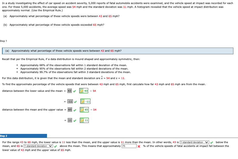
In a study investigating the effect of car speed on accident severity, 5,000 reports of fatal automobile accidents were examined, and the vehicle speed at impact was recorded for each one. For these 5,000 accidents, the average speed was 54 mph and the standard deviation was 11 mph. A histogram revealed that the vehicle speed at impact distribution was approximately normal. (Use the Empirical Rule.) (a) Approximately what percentage of these vehicle speeds were between 43 and 65 mph? (b) Approximately what percentage of these vehicle speeds exceeded 65 mph? Step 1 (a) Approximately what percentage of these vehicle speeds were between 43 and 65 mph? Recall that per the Empirical Rule, if a data distribution is mound shaped and approximately symmetric, then: • Approximately 68% of the observations fall within 1 standard deviation of the mean. Approximately 95% of the observations fall within 2 standard deviations of the mean. Approximately 99.7% of the observations fall within 3 standard deviations of the mean. For this data distribution, it is given that the mean and standard deviation are x = 54 and s = 11. To find the approximate percentage of the vehicle speeds that were between 43 mph and 65 mph, first calculate how far 43 mph and 65 mph are from the mean. distance between the lower value and the mean = 43 43 - 54 -11 -11 distance between the mean and the upper value = 65 65 - 54 11 11 Step 2 For the range 43 to 65 mph, the lower value is 11 less than the mean, and the upper value is 11 more than the mean. In other words, 43 is (1 standard deviation vv below the mean, and 65 is 1 standard deviation v lower value of 43 mph and the upper value of 65 mph. above the mean. This means that approximately 75 X % of the vehicle speeds of fatal accidents at impact fall between the

The mean value of land and buildings per acre from a sample of farms is $1300, with a standard deviation of $100. The data set has a bell-shaped distribution. Using the empirical rule, determine which of the following farms, whose land and building values per acre are given, are unusual (more than two standard deviations from the mean). Are any of the data values very unusual (more than three standard deviations from the mean)? $1321 $1587 $1109 $959 $1492 $1458 Which of the farms are unusual (more than two standard deviations from the mean)? Select all that apply. A. $1587 B. $959 C. $1321 D. $1458 E. $1492 F. $1109

In a study investigating the effect of car speed on accident severity, 5,000 reports of fatal automobile accidents were examined, and the vehicle speed at impact was recorded for each one. For these 5,000 accidents, the average speed was 44 mph and the standard deviation was 17 mph. A histogram revealed that the vehicle speed at impact distribution was approximately normal. (Use the Empirical Rule.) (a) Approximately what percentage of these vehicle speeds were between 27 and 61 mph? approximately  % (b) Approximately what percentage of these vehicle speeds exceeded 61 mph? (Round your answer to the nearest whole number.) approximately  %

In a study investigating the effect of car speed on accident severity, 5,000 reports of fatal automobile accidents were examined, and the vehicle speed at impact was recorded for each one. For these 5,000 accidents, the average speed was 42 mph and the standard deviation was 12 mph. A histogram revealed that the vehicle speed at impact distribution was approximately normal. (Use the Empirical Rule.) (a) Approximately what percentage of vehicle speeds were between 30 and 54 mph? approximately  % (b) Approximately what percentage of vehicle speeds exceeded 54 mph? (Round your answer to the nearest whole number.) approximately  %

An experiment was conducted to determine if exposure to an advertisement would change attitude toward a product. Each subject’s attitude before and after exposure to the advertisement was recorded, using a valid ten point scale. The results indicated: Subject Attitude Post Exposure Attitude Pre Exposure   1 6 4 2 8 5 3 6 6 4 4 3 5 7 2 6 6 3 7 9 6 8 7 6 9 8 5 10 8 6   Set up hypotheses and test to determine if the mean attitude toward the product increased as a result of exposure to the advertisement. (Note: these samples must be regarded as dependent, as each subject served as both a control (pre-exposure) and a treatment (post exposure).   Fully interpret your result.

In a Normal distribution, the Empirical Rule states that...       ["", "", "", "", ""]  of the data is within 1 standard deviation of the mean,       ["", "", "", "", ""]  of the data is within 2 standard deviation of the mean, and       ["", "", "", "", ""]  of the data is within 3 standard deviation of the mean.

light examined data on employment and answered questions regarding why workers separate from their employes. According to the article, the standard deviation of the length of time that women with one job are employed during the first 8 years of their career is 92 weeks. Length of time employed during the first 8 years of career is a left skewed variable. For that variable, do the following tasks. A. determine the sampling distribution of the sample mean for simple random samples of 50 women with one job. Explain your reasoning B. Obtain the probability that the sampling error made in estimating the mean length of time employed by all women with one job by that of a random sample of 50 such women will be at most 20 weeks

The empirical rule states that, for data having a bell-shaped distribution, the percentage of data values being within one standard deviation of the mean is approximately​ a. ​33%. b. ​95%. c. ​68%. d. ​50%.

A study was conducted for an aviation safety agency in which they surveyed thousands of passengers at airports across Europe. In this study, the "mass" for a passenger includes the weight of the passenger and all of the passenger's carry-on items, including infants without their own seats. For the 5,904 adult male passengers measured in summer, the sample mean and standard deviation for this mass were 88.8 kg and 15.9 kg, respectively.   (a) Construct a 95% confidence interval (in kilograms) for the population mean mass for adult male passengers in summer. (Round your answers to three decimal places.) ___to__ kg (b) Write a sentence or two interpreting the confidence interval you found in part (a). With 95% confidence, we can estimate that the population mean mass of male passengers traveling in the summer is contained within the interval. We can estimate that 95% of the male passengers traveling in the summer in the sample have a mass that is contained within the interval.…

The owner of a fish market has an assistant who has determined that the weights of catfish are normally distributed, with a mean of 3.2 pounds and a standard deviation of 0.8 pound. If a sample of 25 fish yields a mean of 3.1 pounds, what is the Z-score for this observation?   Question 3 options:   1)  2.500   2)  0.625   3)  -0.625   4)  1.250