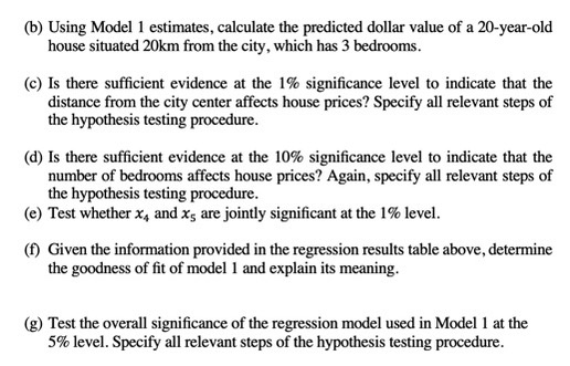
(b) Using Model 1 estimates, calculate the predicted dollar value of a 20-year-oldhouse situated 20km from the city, which has 3 bedrooms.(c) Is there sufficient evidence at the 1% significance level to indicate that thedistance from the city center affects house prices? Specify all relevant steps ofthe hypothesis testing procedure.(d) Is there sufficient evidence at the 10% significance level to indicate that thenumber of bedrooms affects house prices? Again, specify all relevant steps ofthe hypothesis testing procedure.(e) Test whether x, and x5 are jointly significant at the 1% level.(f) Given the information provided in the regression results table above, determinethe goodness of fit of model 1 and explain its meaning.(g) Test the overall significance of the regression model used in Model 1 at the5% level. Specify all relevant steps of the hypothesis testing procedure. Question 2A real estate agent wants to determine the factors that influence house prices inAdelaide. A random sample of 200 houses was selected to estimate the multipleregression model:y =B₁ + B₁x₁ + B₂log(x₂) + B3x3 + B4x4 + Bsxs +uWhere,y = House price (in $10,000s).x₁ = Distance from the city center (in kilometers).x₂ = Number of bedrooms.x3 = Age of the house (in years).X4= Dummy variable equal to 1 if the house has a backyard.x= Proxy for the quality of the neighborhoods' schoolsThe estimation results are shown below when excluding x, and x5 of the regression(Model 1) and when including them (Model 2). Standard errors are in parentheses.Explanatory Variables Model 1Model 2BoB₁B₂B3B₁BsNSSRSST25.3(10.7)-0.032(0.009)15.1(2.3)-1.8(0.5)10043279820.1(15.2)-0.028(0.001)12.4(1.8)-1.5(0.6)5.2(2.1)4.6(1.9)100390798(a) Write down the Sample Regression Function (SRF) for Model 1 in an equationform and interpret each of the estimated slope coefficients.

Given the estimation results when excluding and of the regression (Model 1) and including them…

Answered: A real estate agent wants to determine…

MATLAB: An Introduction with Applications

6th Edition

ISBN:9781119256830

Author:Amos Gilat

Publisher:Amos Gilat

Chapter1: Starting With Matlab

Section: Chapter Questions

Problem 1P

See similar textbooks

Similar questions

What are the interpretations of the Y intercept and the slopes in a multiple regression model?
A biologist wants to predict the height of male giraffes, y, in feet, given their age, x1, in years, weight, x2, in pounds, and neck length, x3, in feet. She obtains the multiple regression equation yˆ=7.36+0.00895x1+0.000426x2+0.913x3. Predict the height of a 12-year-old giraffe that weighs 3,100 pounds and has a 7-foot-long neck, rounding to the nearest foot.
Would the regression in Equation be useful for predicting test scoresin a school district in Massachusetts? Why or why not?
ABC, Inc., sells tea products to various customers. In recent years, profits have been declining. The CFO of the company investigated the reasons for the profit decline and performed regression analysis for sales and costs. She determined that sales depend on product price, delivery speed, customer services, and marketing expenses. She also determined that total costs consist of variable costs of $25 per unit and fixed costs of $56,000. Marketing expenses have a coefficient of determination of 75% related sales.Question: List two advantages and two limitations of regression analysis.
please use this situation: A small theater company has a linear regression model to estimate y = the concession stand sales in dollars, based on knowing x = the number of people in attendance. The regression equation is: = 6.72x + 11.50 and the correlation coefficient was r = 0.781. The data set saw the number of people in attendance ranging from a minimum of 18 people to a maximum of 170 people. 1) How reliable would it be to make a prediction for the concession sales amount if there were 500 people in attendance? Explain.
La Quinta Inns has a competitive edge over its rivals because it: uses regression analysis to determine which variables most influence profitability. has better television advertisements. picks larger locations than its rivals. builds only along interstate highways. consistently receives four-star ratings for its inns.
The accompanying table shows results from regressions performed on data from a random sample of 21 cars. The response (y) variable is CITY (fuel consumption in mi/gal). The predictor (x) variables are WT (weight in pounds), DISP (engine displacement in liters), and HWY (highway fuel consumption in mi/gal). The equation CITY - 3.17 +0.823HWY was previously determined to be the best for predicting city fuel consumption. A car weighs 2700 lb, it has an engine displacement of 1.6 L, and its highway fuel consumption is 35 mi/gal. What is the best predicted value of the city fuel consumption? Is that predicted value likely to be a good estimate? Is that predicted value likely to be very accurate? Click the icon to view the table of regression equations. The best predicted value of the city fuel consumption is (Type an integer or a decimal. Do not round.). Regression Table I R² Adjusted R2 WT/DISP WT/HWY Predictor (x) Variables P-Value WT/DISP/HWY 0.000 0.942 0.000 0.748 0.000 0.942 0.000…
A real estate analyst has developed a multiple regression line, y = 60 + 0.068 x1 – 2.5 x2, to predict y = the market price of a home (in $1,000s), using two independent variables, x1 = the total number of square feet of living space, and x2 = the age of the house in years. With this regression model, the predicted price of a 10-year old home with 2,500 square feet of living area is __________. $205.00 $200,000.00 $205,000.00 $255,000.00
Range of ankle motion is a contributing factor to falls among the elderly. Suppose a team of researchers is studying how compression hosiery, typical shoes, and medical shoes affect range of ankle motion. In particular, note the variables Barefoot and Footwear2. Barefoot represents a subject's range of ankle motion (in degrees) while barefoot, and Footwear2 represents their range of ankle motion (in degrees) while wearing medical shoes. Use this data and your preferred software to calculate the equation of the least-squares linear regression line to predict a subject's range of ankle motion while wearing medical shoes, ?̂ , based on their range of ankle motion while barefoot, ? . Round your coefficients to two decimal places of precision. ?̂ = A physical therapist determines that her patient Jan has a range of ankle motion of 7.26°7.26° while barefoot. Predict Jan's range of ankle motion while wearing medical shoes, ?̂ . Round your answer to two decimal places. ?̂ = Suppose Jan's…
In a fisheries researchers experiment the correlation between the number of eggs in tge nest and the number of viable (surviving ) eggs for a sample of nests is r=0.67 the equation of the regression line for number of viable eggs y versus number of eggs in the nest x is y =0.72x + 17.07 for a nest with 140 eggs what is the predicted number of viable eggs ?
For 50 students of a class the regression equation of marks in Statistics (X) on the marks in Accountancy (Y) is 3Y – 5 X + 180 = 0. The mean marks of Accountancy is 44 and variance of marks in Statistics is 9/16th of the variance of marks in Accountancy. Find the mean marks of Statistics and the coefficient of correlation between marks in two subjects.
The best-predicted weight for a bear with a chest of 44 inches is how many pounds? Is the close to the actual weight of 293 pounds?

Recommended textbooks for you

MATLAB: An Introduction with Applications

Statistics

ISBN:

9781119256830

Author:

Amos Gilat

Publisher:

John Wiley & Sons Inc

Probability and Statistics for Engineering and th…

Statistics

ISBN:

9781305251809

Author:

Jay L. Devore

Publisher:

Cengage Learning

Statistics for The Behavioral Sciences (MindTap C…

Statistics

ISBN:

9781305504912

Author:

Frederick J Gravetter, Larry B. Wallnau

Publisher:

Cengage Learning

MATLAB: An Introduction with Applications

Statistics

ISBN:

9781119256830

Author:

Amos Gilat

Publisher:

John Wiley & Sons Inc

Probability and Statistics for Engineering and th…

Statistics

ISBN:

9781305251809

Author:

Jay L. Devore

Publisher:

Cengage Learning

Statistics for The Behavioral Sciences (MindTap C…

Statistics

ISBN:

9781305504912

Author:

Frederick J Gravetter, Larry B. Wallnau

Publisher:

Cengage Learning

Elementary Statistics: Picturing the World (7th E…

Statistics

ISBN:

9780134683416

Author:

Ron Larson, Betsy Farber

Publisher:

PEARSON

The Basic Practice of Statistics

Statistics

ISBN:

9781319042578

Author:

David S. Moore, William I. Notz, Michael A. Fligner

Publisher:

W. H. Freeman

Introduction to the Practice of Statistics

Statistics

ISBN:

9781319013387

Author:

David S. Moore, George P. McCabe, Bruce A. Craig

Publisher:

W. H. Freeman

SEE MORE TEXTBOOKS