
MATLAB: An Introduction with Applications
6th Edition
ISBN: 9781119256830
Author: Amos Gilat
Publisher: John Wiley & Sons Inc
expand_more
expand_more
format_list_bulleted
Related questions
Concept explainers
Topic Video
Question
Find the equation of the regression line for the given data. Then construct a
y^=[ ]x +([ ])
(Round the slope to three decimal places as needed. Round the y-intercept to two decimal places as needed.)
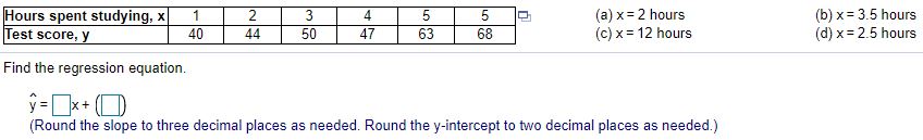

Transcribed Image Text:Hours spent studying, x
Test score, y
(a) x= 2 hours
(c) x = 12 hours
(b) x= 3.5 hours
(d) x= 2.5 hours
1
2
3
4
40
44
50
47
63
68
Find the regression equation.
ý=*+ (O
(Round the slope to three decimal places as needed. Round the y-intercept to two decimal places as needed.)
Expert Solution
This question has been solved!
Explore an expertly crafted, step-by-step solution for a thorough understanding of key concepts.

This is a popular solution

Trending nowThis is a popular solution!

Step by stepSolved in 4 steps with 9 images

Knowledge Booster


Learn more about
Need a deep-dive on the concept behind this application? Look no further. Learn more about this topic, statistics and related others by exploring similar questions and additional content below.Similar questions
- The equation used to predict annual cauliflower yield (in pounds per acre) is y=24,786+4.563x, -4.736x2, where x, is the number of acres planted and x₂ is the number of acres harvested. Use the multiple regression equation to predict the y-values for the values of the independent variables. (a) x, 37,000, x₂=37,400 (b)x₁=38,700, x₂ = 39,000 (c) x₁=39,700, x₂-39,900 (d) x, 43,000, x₂=43,100 (a) The predicted yield is pounds per acre. (Round to one decimal place as needed.) CITarrow_forwardIf the linear equation between Height and Gestational Age is given as: Height=a + b Gest x What is the value of a from the output above What is the value of b from the output abovearrow_forward- X Wins and ERA Earned run Wins, x average, y 20 2.79 18 3.31 17 2.65 16 3.83 14 3.94 12 4.27 11 3.78 9 5.18 Print Donearrow_forward
- Given that the systolic blood pressure in the right arm is 90 mm Hg, the best systolic blood pressure in the left arm is how many mm Hg?arrow_forwardSelect the appropriate interpretation for the slope of the linear regression equation below. Y (Dependent Variable) = Grade Point Average X (Independent Variable) = Average number of hours spent using electronic devices for entertainment purposes yhat = 4 - 0.125*X A. For every 1 hour more spent using electronic devices for entertainment per week then a person's GPA will increase on average by 0.125 points B. For every 1 GPA gained obtained by a student then on average that person will have watched 0.125 hours fewer of entertainment on electronic devices per week C. For every 1 GPA point lost by a student then on average that person will have watched 0.125 hours more of entertainment on electronic devices per week D. For every 1 hour more spent using electronic devices for entertainment per week then a person's GPA will decrease on average by 0.125 pointsarrow_forwardShow the best fitted line on scatter diagram and Find the predicted value for each y using the exposure time and the equation obtained in part b (b. Find the equation of regression line between radiation doses on exposure time .usingleast square method)arrow_forward
- A box office analyst seeks to predict opening weekend box office gross for movies. Toward this goal, the analyst plans to use online trailer views as a predictor. For each of the 66 movies, the number of online trailer views from the release of the trailer through the Saturday before a movie opens and the opening weekend box office gross (in millions of dollars) are collected and stored in the accompanying table. A linear regression was performed on these data, and the result is the linear regression equation Yi=−0.840+1.4108Xi. Determine the coefficient of determination,r2,and interpret its meaning. Determine the standard error of the estimate. How useful do you think this regression model is for predicting opening weekend box office gross? Can you think of other variables that might explain the variation in opening weekend box office gross?arrow_forwardA box office analyst seeks to predict opening weekend box office gross for movies. Toward this goal, the analyst plans to use online trailer views as a predictor. For each of the 66 movies, the number of online trailer views from the release of the trailer through the Saturday before a movie opens and the opening weekend box office gross (in millions of dollars) are collected and stored in the accompanying table. A linear regression was performed on these data, and the result is the linear regression equation Yi=−1.254+1.3968Xi. Complete parts (a) through (d). a. Determine the coefficient of determination,r2,and interpret its meaning. b. Determine the standard error of the estimate. c. How useful do you think this regression model is for predicting opening weekend box office gross? d. Can you think of other variables that might explain the variation in opening weekend box office gross?arrow_forwardA financial website reported the beta value for a certain company was 0.86. Betas for individual stocks are determined by simple linear regression. The dependent variable is the total return for the stock, and the independent variable is the total return for the stock market, such as the return of a market index. The slope of this regression equation is referred to as the stock's beta. Many financial analysts prefer to measure the risk of a stock by computing the stock's beta value. Suppose the following data show the monthly percentage returns for the market index and the company for a recent year. Month Market Index% Return Company% Return August -3 4 September 8 7 October 0 1 November -2 1 December -5 0 January 0 0 February 7 7 March 0 -2 April 2 0 May -5 -1 a. Develop the least squares estimated regression equation. (Let x = Market Index % Return (as a %), and let y = Company % Return (as a %). Round your numerical values to four decimal places.)arrow_forward
- A particular article used a multiple regression model to relate y = yield of hops to x₁ = mean temperature (°C) between date of coming into hop and date of picking and x₂ = mean percentage of sunshine during the same period. The model equation proposed is the following. y = 415.116.6x₁4.50x2+e (a) Suppose that this equation does indeed describe the true relationship. What mean yield corresponds to a temperature of 20 and a sunshine percentage of 39? (b) What is the mean yield when the mean temperature and percentage of sunshine are 19.1 and 42, respectively? You may need to use the appropriate table in Appendix A to answer this question.arrow_forwardThe accompanying data are the number of wins and the earned run averages (mean number of earned runs allowed per nine innings pitched) for eight baseball pitchers in a recent season. Find the equation of the regression line. Then construct a scatter plot of the data and draw the regression line. Then use the regression equation to predict the value of y for each of the given x-values, if meaningful. If the x-value is not meaningful to predict the value of y, explain why not. (a) x = 5 wins Click the icon to view the table of numbers of wins and earned run average. (b) x= 10 wins (c) x=21 wins (d) x= 15 wins The equation of the regression line is y = x+ | (Round to two decimal places as needed.) !!arrow_forwardIn calculating a simple regression for average number of drinks consumed (x) and grade point average (y), you get a slope coefficient (b) of -.15 and a y intercept of 2.50. Using the formula Y = a + bX, what would the predicted grade point average be for a student who averaged 1.0 drinks per week?arrow_forward
arrow_back_ios
arrow_forward_ios
Recommended textbooks for you
- MATLAB: An Introduction with ApplicationsStatisticsISBN:9781119256830Author:Amos GilatPublisher:John Wiley & Sons Inc
 Probability and Statistics for Engineering and th...StatisticsISBN:9781305251809Author:Jay L. DevorePublisher:Cengage Learning
 Statistics for The Behavioral Sciences (MindTap C...StatisticsISBN:9781305504912Author:Frederick J Gravetter, Larry B. WallnauPublisher:Cengage Learning
  Elementary Statistics: Picturing the World (7th E...StatisticsISBN:9780134683416Author:Ron Larson, Betsy FarberPublisher:PEARSON
 The Basic Practice of StatisticsStatisticsISBN:9781319042578Author:David S. Moore, William I. Notz, Michael A. FlignerPublisher:W. H. Freeman
 Introduction to the Practice of StatisticsStatisticsISBN:9781319013387Author:David S. Moore, George P. McCabe, Bruce A. CraigPublisher:W. H. Freeman
MATLAB: An Introduction with Applications
Statistics
ISBN:9781119256830
Author:Amos Gilat
Publisher:John Wiley & Sons Inc
Probability and Statistics for Engineering and th...
Statistics
ISBN:9781305251809
Author:Jay L. Devore
Publisher:Cengage Learning
Statistics for The Behavioral Sciences (MindTap C...
Statistics
ISBN:9781305504912
Author:Frederick J Gravetter, Larry B. Wallnau
Publisher:Cengage Learning
Elementary Statistics: Picturing the World (7th E...
Statistics
ISBN:9780134683416
Author:Ron Larson, Betsy Farber
Publisher:PEARSON
The Basic Practice of Statistics
Statistics
ISBN:9781319042578
Author:David S. Moore, William I. Notz, Michael A. Fligner
Publisher:W. H. Freeman
Introduction to the Practice of Statistics
Statistics
ISBN:9781319013387
Author:David S. Moore, George P. McCabe, Bruce A. Craig
Publisher:W. H. Freeman