
MATLAB: An Introduction with Applications
6th Edition
ISBN: 9781119256830
Author: Amos Gilat
Publisher: John Wiley & Sons Inc
expand_more
expand_more
format_list_bulleted
Related questions
Question
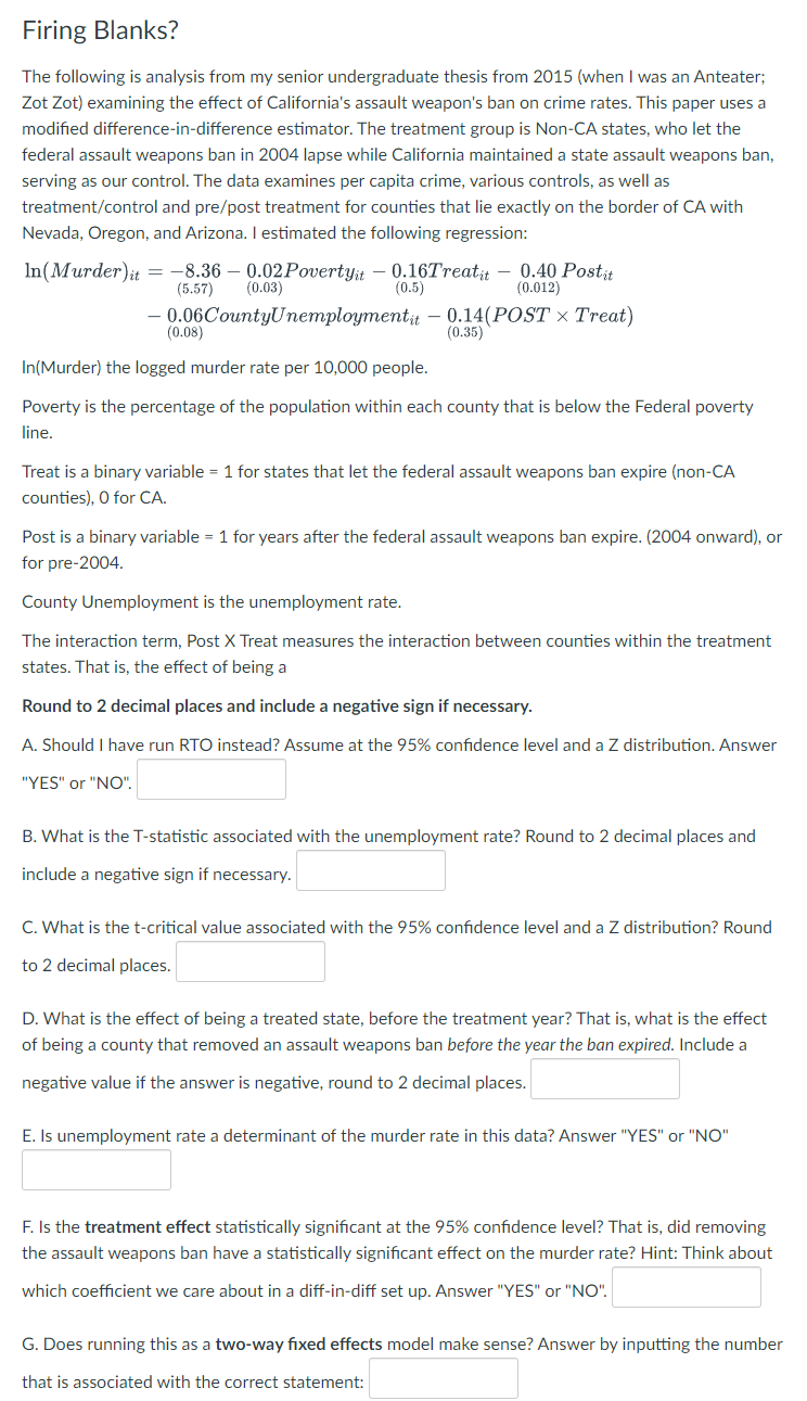

Transcribed Image Text:Firing Blanks?
The following is analysis from my senior undergraduate thesis from 2015 (when I was an Anteater;
Zot Zot) examining the effect of California's assault weapon's ban on crime rates. This paper uses a
modified difference-in-difference estimator. The treatment group is Non-CA states, who let the
federal assault weapons ban in 2004 lapse while California maintained a state assault weapons ban,
serving as our control. The data examines per capita crime, various controls, as well as
treatment/control and pre/post treatment for counties that lie exactly on the border of CA with
Nevada, Oregon, and Arizona. I estimated the following regression:
In(Murder) it = -8.36 0.02Povertyit -0.16Treatit - 0.40 Postit
(5.57) (0.03)
(0.5)
(0.012)
-0.06CountyUnemploymentit 0.14(POST X Treat)
(0.35)
(0.08)
In(Murder) the logged murder rate per 10,000 people.
Poverty is the percentage of the population within each county that is below the Federal poverty
line.
Treat is a binary variable = 1 for states that let the federal assault weapons ban expire (non-CA
counties), O for CA.
Post is a binary variable = 1 for years after the federal assault weapons ban expire. (2004 onward), or
for pre-2004.
County Unemployment is the unemployment rate.
The interaction term, Post X Treat measures the interaction between counties within the treatment
states. That is, the effect of being a
Round to 2 decimal places and include a negative sign if necessary.
A. Should I have run RTO instead? Assume at the 95% confidence level and a Z distribution. Answer
"YES" or "NO".
B. What is the T-statistic associated with the unemployment rate? Round to 2 decimal places and
include a negative sign if necessary.
C. What is the t-critical value associated with the 95% confidence level and a Z distribution? Round
to 2 decimal places.
D. What is the effect of being a treated state, before the treatment year? That is, what is the effect
of being a county that removed an assault weapons ban before the year the ban expired. Include a
negative value if the answer is negative, round to 2 decimal places.
E. Is unemployment rate a determinant of the murder rate in this data? Answer "YES" or "NO"
F. Is the treatment effect statistically significant at the 95% confidence level? That is, did removing
the assault weapons ban have a statistically significant effect on the murder rate? Hint: Think about
which coefficient we care about in a diff-in-diff set up. Answer "YES" or "NO".
G. Does running this as a two-way fixed effects model make sense? Answer by inputting the number
that is associated with the correct statement:

Transcribed Image Text:Post is a binary variable = 1 for years after the federal assault weapons ban expire. (2004 onward), or
for pre-2004.
County Unemployment is the unemployment rate.
The interaction term, Post X Treat measures the interaction between counties within the treatment
states. That is, the effect of being a
Round to 2 decimal places and include a negative sign if necessary.
A. Should I have run RTO instead? Assume at the 95% confidence level and a Z distribution. Answer
"YES" or "NO".
B. What is the T-statistic associated with the unemployment rate? Round to 2 decimal places and
include a negative sign if necessary.
C. What is the t-critical value associated with the 95% confidence level and a Z distribution? Round
to 2 decimal places.
D. What is the effect of being a treated state, before the treatment year? That is, what is the effect
of being a county that removed an assault weapons ban before the year the ban expired. Include a
negative value if the answer is negative, round to 2 decimal places.
E. Is unemployment rate a determinant of the murder rate in this data? Answer "YES" or "NO"
F. Is the treatment effect statistically significant at the 95% confidence level? That is, did removing
the assault weapons ban have a statistically significant effect on the murder rate? Hint: Think about
which coefficient we care about in a diff-in-diff set up. Answer "YES" or "NO".
G. Does running this as a two-way fixed effects model make sense? Answer by inputting the number
that is associated with the correct statement:
1. No, because there really shouldn't be anything different between bordering counties in CA
and counties in Nevada, Arizona, or Oregon
2. No, because we only really need to account for county level differences in CA, Nevada,
Arizona, and Oregon
3. No, because we only really need to account for how murder changes over time
4. Yes, because crime probably has a time trend component that is fixed across counties as well
as having some unobserved fixed characteristics between counties that we should account
for.
5. Yes, because we need to control for simultaneity --- did the state pass assault weapons ban in
response to higher crime or did the crime rate respond to the passage of the assault weapons
ban?
H. Suppose that you believe that undergraduate Harrison was an idiot and omitted the variable
education. You also know:
Cov(Educ, Poverty) < 0
Cov(Educ, Murder) < 0
What is the direction of the bias on the coefficient for Poverty? Answer "UPWARD" or
"DOWNWARD"
Expert Solution
This question has been solved!
Explore an expertly crafted, step-by-step solution for a thorough understanding of key concepts.

This is a popular solution

Trending nowThis is a popular solution!

Step by stepSolved in 3 steps

Knowledge Booster

Similar questions
- The authors of a paper describe an experiment to evaluate the effect of using a cell phone on reaction time. Subjects were asked to perform a simulated driving task while talking on a cell phone. While performing this task, occasional red and green lights flashed on the computer screen. If a green light flashed, subjects were to continue driving, but if a red light Flashed, subjects were to brake as quickly as possible. The reaction time (in msec) was recorded. The following summary statistics are based on a graph that appeared in the paper. n = 49 x = 530 S = 65 USE SALT (a) Construct a 95% confidence interval for u, the mean time to react to a red light while talking on a cell phone. (Round your answers to three decimal places.) Interpret a 95% confidence interval for μ, the mean time to react to a red light while talking on a cell phone. We are 95% confident that the mean time to react to a red light while talking on a cell phone is between these two values. There is a 95% chance…arrow_forward20 Total 58 11. The following summary table presents the results from an ANOVA comparing four treatment conditions with n = 10 participants in each condition. Complete all missing values. (Hint: Start with the df column.) 15 Source SS df MS Between treatments 10 F =_ Within treatments Total 16. 174 opment of language skills from age 2 to age 4. Three Lis en are obtained, one for each 12. A is the devel-arrow_forwardEducation influences attitude and lifestyle. Differences in education are a big factor in the "generation gap." Is the younger generation really better educated? Large surveys of people age 65 and older were taken in n1 = 38 U.S. cities. The sample mean for these cities showed that x1 = 15.2% of the older adults had attended college. Large surveys of young adults (age 25 - 34) were taken in n2 = 37 U.S. cities. The sample mean for these cities showed that x2 = 18.1% of the young adults had attended college. From previous studies, it is known that ?1 = 6.4% and ?2 = 4.8%. Does this information indicate that the population mean percentage of young adults who attended college is higher? Use ? = 0.05. What is the value of the sample test statistic? (Test the difference ?1 − ?2. Round your answer to two decimal places.)=__(c) Find (or estimate) the P-value. (Round your answer to four decimal places.)=__arrow_forward
- can you please help me with my stats homework?arrow_forwardA company has 25 applicants to interview, and wants to invite 7 of them on the first day, 6 of them on the second day, 5 of them on the third day, 4 of them on the fourth day and 3 of them on the fifth day of a week. In how many ways can the applicants be scheduled? Select one: (257,6,5,4,3) None 25! P(25;7)xP(19;6) ×P(14;5)xP(10;4)×P(7;3) C(25;7)xC(19;6)xC(14;5)xC(10;4)xC(7;3)arrow_forwardThe GHQ is a well-known instrument for measuring minor psychological distress. The scale asks whether the respondent has experienced a particular symptom or behavior recently. Higher scores are associated with worst mental health. Past research has demonstrated that being of lower socioeconomic status was also associated with poorer mental health. The data are below: Participant Financial Security GHQ 1 20 25 2 18 23 3 18 17 4 19 35 5 19 18 6 18 24 7 19 24 8 14 25 9 10 27 10 7 50 i just need help on the blanks in the picture thankyouarrow_forward
- Read the scenario below to determine which one of the time threats to internal validity (test reactivity, instrumentation, history, and maturation) is of most concern, and provide one way to control for the threat. A researcher examines students' perception of their body image by conducting a 2-year longitudinal study of middle-school students (grades 6 - 8). Body image is measured using a scale and the same scale is measured under the same conditions at the beginning and end of the study.arrow_forwardStudy 2: Pill Appearance and Perceived Pain. Does the shape or color of a pain pill influence its effectiveness? Although logically it shouldn’t, whether we believe a drug will work does have a powerful effect on our perceptions (e.g., placebo effect). In this experiment, 4 groups of adult patients were given the same amount of Advil after dental surgery for pain relief, but the color and shape of the pill varied. Researchers hypothesized that an unusual shape or color would lead people to believe the pills were new and special and thus would expect them to be more effective than common round, white pills. Researchers also wanted to know if there is an interaction between shape and color Data Labels ShapePill {1=Round; 2=Diamond} ColorPill {1=White; 2=BlueGreen} Gender {0=Woman; 1=Man; 2=Nonbinary person) Descriptions of the Variables and Descriptive Statistics: Referring to the JASP output, and using sentences, present the descriptive statistics of each group: for example:…arrow_forwardThe phrase “Correlation does not equal causation” means: Question 30 options: there is no guarantee that a cause-and-effect relationship exists between two variables that are correlated. there is only a 30% chance that a cause-and-effect relationship exists between two variables. a cause-and-effect relationship only certainly exists when data are gathered in a specific way. a cause-and-effect relationship can only exist with ratio-level variables.arrow_forward
- A survey collected data on annual credit card charges in seven different categories of expenditures: transportation, groceries, dining out, household expenses, home furnishings, apparel, and entertainment. Using data from a sample of 42 credit card accounts, assume that each account was used to identify the annual credit card charges for groceries (population 1) and the annual credit card charges for dining out (population 2). Using the difference data, with population 1– population 2, the sample mean difference was d = $870, and the sample standard deviation was s,= $1,125. (a) Formulate the null and alternative hype to test for no difference between the population mean credit card charges for groceries and the population mean credit card charges for dining out. 0> Prt :°H 0 = Pri :ºH O O Ho: Hdso H: H=0 (b) Calculate the test statistic. (Round your answer to three decimal places.) What is the p-value? (Round your answer to four decimal places.) Can you conclude that the population…arrow_forwardRewrite the following sentence to remove its primary problem "We hypothesize that grade level has an effect on academic success."arrow_forwardEducation influences attitude and lifestyle. Differences in education are a big factor in the "generation gap." Is the younger generation really better educated? Large surveys of people age 65 and older were taken in n1 = 38 U.S. cities. The sample mean for these cities showed that x1 = 15.2% of the older adults had attended college. Large surveys of young adults (age 25 - 34) were taken in n2 = 37 U.S. cities. The sample mean for these cities showed that x2 = 18.1% of the young adults had attended college. From previous studies, it is known that ?1 = 6.4% and ?2 = 4.8%. Does this information indicate that the population mean percentage of young adults who attended college is higher? Use ? = 0.05. (c) Find (or estimate) the P-value. (Round your answer to four decimal places.) A random sample of n1 = 12 winter days in Denver gave a sample mean pollution index x1 = 43. Previous studies show that ?1 = 15. For Englewood (a suburb of Denver), a random sample of n2 = 16 winter days gave a…arrow_forward
arrow_back_ios
SEE MORE QUESTIONS
arrow_forward_ios
Recommended textbooks for you
- MATLAB: An Introduction with ApplicationsStatisticsISBN:9781119256830Author:Amos GilatPublisher:John Wiley & Sons Inc
 Probability and Statistics for Engineering and th...StatisticsISBN:9781305251809Author:Jay L. DevorePublisher:Cengage Learning
 Statistics for The Behavioral Sciences (MindTap C...StatisticsISBN:9781305504912Author:Frederick J Gravetter, Larry B. WallnauPublisher:Cengage Learning
  Elementary Statistics: Picturing the World (7th E...StatisticsISBN:9780134683416Author:Ron Larson, Betsy FarberPublisher:PEARSON
 The Basic Practice of StatisticsStatisticsISBN:9781319042578Author:David S. Moore, William I. Notz, Michael A. FlignerPublisher:W. H. Freeman
 Introduction to the Practice of StatisticsStatisticsISBN:9781319013387Author:David S. Moore, George P. McCabe, Bruce A. CraigPublisher:W. H. Freeman
MATLAB: An Introduction with Applications
Statistics
ISBN:9781119256830
Author:Amos Gilat
Publisher:John Wiley & Sons Inc
Probability and Statistics for Engineering and th...
Statistics
ISBN:9781305251809
Author:Jay L. Devore
Publisher:Cengage Learning
Statistics for The Behavioral Sciences (MindTap C...
Statistics
ISBN:9781305504912
Author:Frederick J Gravetter, Larry B. Wallnau
Publisher:Cengage Learning
Elementary Statistics: Picturing the World (7th E...
Statistics
ISBN:9780134683416
Author:Ron Larson, Betsy Farber
Publisher:PEARSON
The Basic Practice of Statistics
Statistics
ISBN:9781319042578
Author:David S. Moore, William I. Notz, Michael A. Fligner
Publisher:W. H. Freeman
Introduction to the Practice of Statistics
Statistics
ISBN:9781319013387
Author:David S. Moore, George P. McCabe, Bruce A. Craig
Publisher:W. H. Freeman