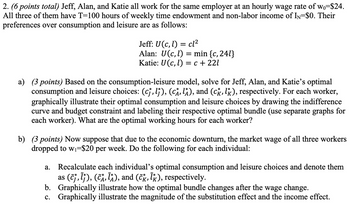
2. (6 points total) Jeff, Alan, and Katie all work for the same employer at an hourly wage rate of wo=$24. All three of them have T=100 hours of weekly time endowment and non-labor income of IN=$0. Their preferences over consumption and leisure are as follows: Jeff: U(c, l) = cl² Alan: U(c,l) = min {c, 241} Katie: U (c, l) = c +221 a) (3 points) Based on the consumption-leisure model, solve for Jeff, Alan, and Katie's optimal consumption and leisure choices: (cj, lj), (CA, lA), and (ck, lk), respectively. For each worker, graphically illustrate their optimal consumption and leisure choices by drawing the indifference curve and budget constraint and labeling their respective optimal bundle (use separate graphs for each worker). What are the optimal working hours for each worker? b) (3 points) Now suppose that due to the economic downturn, the market wage of all three workers dropped to w₁-$20 per week. Do the following for each individual: a. Recalculate each individual's optimal consumption and leisure choices and denote them as (ĉƒ‚Ã), (ĉ ÎÂ), and (čk, Îk), respectively. b. Graphically illustrate how the optimal bundle changes after the wage change. c. Graphically illustrate the magnitude of the substitution effect and the income effect.