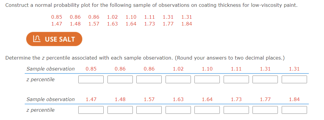
Construct a normal probability plot for the following sample of observations on coating thickness for low-viscosity paint. 0.85 0.86 0.86 1.02 1.10 1.11 1.31 1.31 1.47 1.48 1.57 1.63 1.64 1.73 1.77 1.84 USE SALT Determine the z percentile associated with each sample observation. (Round your answers to two decimal places.) Sample observation 0.85 0.86 1.11 z percentile Sample observation z percentile 1.47 1.48 0.86 1.57 1.02 1.63 1.10 1.64 1.73 1.31 1.77 1.31 1.84

b. Sketch a standard normal curve and shade the area under the curve that lies between - 3 and - 2.1. Choose the correct graph below. А. В. С. OD. - 2.1 2.1 O 2.1 3 O 2.1 3 The area that lies between - 3 and - 2.1 is 0.98 (Round to four decimal places as needed.) N

Which way of dispensing champagne, the traditional vertical method or a tilted beer-like pour, preserves more of the tiny gas bubbles that improve flavor and aroma? The following data was reported in an article. Type of Pour n Mean (g/L) SD 0.6 Traditional 4 Slanted Traditional 4 0.4 0.2 Slanted 4 0.1 Assume that the sampled distributions are normal. Temp (°C) 18 18 12 12 LUSE SALT (a) Carry out a test at significance level 0.01 to decide whether true average CO₂, loss at 18°C for the traditional pour differs from that for the slanted pour. (Use μ, for the traditional pour and State the relevant hypotheses. OH₂H₂H₂ 0 OHH₁-H₂0 H₂H₁-H₂=0 OH₂H₁ H₂=0 H₂H₁ H₂ <0 (b) Repeat the test of hypotheses suggested in (a) for the 12° temperature. Is the conclusion different from that for the 18° temperature? Note: The 12° result was reported in the popular media. (Use u, for the traditional pour and for the slanted pour.) State the relevant hypotheses. OHH, H₂ <0 H₂₁₂4₁₂4₂₁₂=0 - OH₂H₁-H₂=0 H₂H₂H₂ #0…

Construct a normal probability plot for the following sample of observations on coating thickness for low-viscosity paint. 0.82 0.87 0.90 1.02 1.11 1.14 1.31 1.33 1.47 1.48 1.61 1.63 1.64 1.72 1.74 1.84 Determine the z percentile associated with each sample observation. (Round your answers to two decimal places.) Sample observation 0.82 0.87 0.90 1.02 1.11 1.14 1.31 1.33 z percentile Sample observation 1.47 1.48 1.61 1.63 1.64 1.72 1.74 1.84 z percentile

An FDA representative randomly selects 88 packages of ground chuck from a grocery store and measures the fat content (as a percent) of each package. Assume that the fat contents have an approximately normal distribution. The resulting measurements are given below. Fat Contents (%) 12 15 16 13 15 13 15 13 Copy Data   Step 1 of 2 :   Calculate the sample mean and the sample standard deviation of the fat contents. Round your answers to two decimal places, if necessary

Consider the following sample of observations on coating thickness for low-viscosity paint. 0.83   0.88   0.88   1.03   1.09   1.21   1.29   1.31 1.42   1.49   1.59   1.62   1.65   1.71   1.76   1.83 Assume that the distribution of coating thickness is normal (a normal probability plot strongly supports this assumption). (c) Calculate a point estimate of the value that separates the largest 10% of all values in the thickness distribution from the remaining 90%. [Hint: Express what you are trying to estimate in terms of μ and σ.] (Round your answer to four decimal places.)   (d) Estimate P(X < 1.2), i.e., the proportion of all thickness values less than 1.2. [Hint: If you knew the values of μ and σ, you could calculate this probability. These values are not available, but they can be estimated.] (Round your answer to four decimal places.)   (e) What is the estimated standard error of the estimator that you used in part (b)? (Round your answer to four decimal places.)

Construct a normal probability plot for the following sample of observations on coating thickness for low-viscosity paint. 0.84 0.89 0.90 1.02 1.08 1.14 1.28 1.31 1.47 1.47 1.60 1.62 1.66 1.73 1.75 1.81 Determine the z percentile associated with each sample observation. (Round your answers to two decimal places.) Sample observation 0.84 0.89 0.90 1.02 1.08 1.14 1.28 1.31 z percentile                     Sample observation 1.47 1.47 1.60 1.62 1.66 1.73 1.75 1.81 z percentile