choices for the numebred blanks are 1. falling or rising2. falling or rising 3. falling or rising 4. at its maximum, when the avaerage total cost is at 0, or, at its minimum pls also answer the rest of the questions and the graphs. thank you!! On the following graph, use the orange points (square symbol) to plot Felix's free-throw percentage for each game individually, and use the greenpoints (triangle symbol) to plot his overall average free-throw percentage after each game.Note: Plot your points in the order in which you would like them connected. Line segments will connect the points automatically.(?)10090Game Free-Throw Percentage807060Average Free-Throw Percentage5040302010123GAMEYou can think of the result in any one game as being Felix's marginal free-throw percentage. Based on your previous answer, you can deduce thatwhen Felix's marginal free-throw percentage is above the average, the average must beYou can now apply this analysis to production costs. For a U-shaped average total cost curve, when the marginal cost curve is below the average totalcost curve, the average total cost must be 2cost must be ▼. Therefore, the marginal cost curve intersects the average total cost curveAlso, when the marginal cost curve is above the average total cost curve, the average totalFREE-THROW PERCENTAGE Consider the following scenario to understand the relationship between marginal and average values. Suppose Felix is a professional basketball player,and his game log for free throws can be summarized in the following table.Fill in the columns with Felix's free-throw percentage for each game and his overall free-throw average after each game.GameGame ResultTotalGame Free-Throw PercentageAverage Free-Throw Percentage16/86/8757522/88/1632/410/208/1018/3058/1026/40On the following graph, use the orange points (square symbol) to plot Felix's free-throw percentage for each game individually, and use the greenpoints (triangle symbol) to plot his overall average free-throw percentage after each game.Note: Plot your points in the order in which you would like them connected. Line segments will connect the points automatically.10090Game Free-Throw Percentage807060Average Free-Throw Percentage5040E-THROW PERCENTAGE

Answered: Image /qna-images/answer/a8f97108-f7af-4bee-a6a0-0a3719d120dd.jpg

Consider the following scenario to understand the relationship between marginal and average values. Suppose Felix is a professional basketball player, and his game log for free throws can be summarized in the following table. Fill in the columns with Felix's free-throw percentage for each game and his overall free-throw average after each game. Game Game Result Total Game Free-Throw Percentage Average Free-Throw Percentage 1 6/8 6/8 75 75 2/8 8/16 3 2/4 10/20 4 8/10 18/30 5 8/10 26/40 On the following graph, use the orange points (square symbol) to plot Felix's free-throw percentage for each game individually, and use the green points (triangle symbol) to plot his overall average free-throw percentage after each game. Note: Plot your points in the order in which you would like them connected. Line segments will connect the points automatically. 100 90 Game Free-Throw Percentage 80 70 60 Average Free-Throw Percentage 50 40 THROW PERCEN TAGE

Consider the following scenario to understand the relationship between marginal and average values. Suppose Felix is a professional basketball player, and his game log for free throws can be summarized in the following table. Fill in the columns with Felix's free-throw percentage for each game and his overall free-throw average after each game. Game Game Result Total Game Free-Throw Percentage Average Free-Throw Percentage 1 6/8 6/8 75 75 2/8 8/16 3 2/4 10/20 4 8/10 18/30 5 8/10 26/40 On the following graph, use the orange points (square symbol) to plot Felix's free-throw percentage for each game individually, and use the green points (triangle symbol) to plot his overall average free-throw percentage after each game. Note: Plot your points in the order in which you would like them connected. Line segments will connect the points automatically. 100 90 Game Free-Throw Percentage 80 70 60 Average Free-Throw Percentage 50 40 THROW PERCEN TAGE

MATLAB: An Introduction with Applications

6th Edition

ISBN:9781119256830

Author:Amos Gilat

Publisher:Amos Gilat

Chapter1: Starting With Matlab

Section: Chapter Questions

Problem 1P

See similar textbooks

Related questions

Q: Can someone please help to make the graph and answer the question? Sample with the 1 m² and the…

A: In this problem, we have collected data on the number of plant species found in 1 m² and 16 m²…

Q: what is the total distance traveled during the walk represented by the speed versus time graph below

A: Given, The graph of speed versus time. We have to find the total distance traveled during the walk.…

Q: find stem and leaf graphs and box pilot (and box and whisker) and interpretation

A: The data is as follows: Price/TL 25.2795 39.95 4215 572 1407 9754 35898

Q: Uptown Printing CA Mid-City Printers СА Above are the graphs of the Cost, c, of ordering n wedding…

Q: Analysis - Part 2: Make a graph of volume of water vs mass of water (make sure to label each axis…

Q: Findings: Data was skewed to the right The percentage of kids watching tv 4-5 hours a day was 0.4…

A: The data contain name of kids, how nay years they old and hours time watching TV are given…

Q: Jamila has a weather station in her backyard. She uses a rain gauge to track the total rainfall…

Q: Amount Earned ($) 0. 10 30 40 50 "he graph shows the earning from a bake sale per item sold Vhich…

Q: 3. Graph the following equations. State the slope. a. x = 2 EAP EAT 306418 b. y = - 1 CAP Eduation…

A: “Since you have posted multiple questions, we will provide the solution only to the first question…

Q: Use the graph to complete parts (a) and (b) below. 800- 700- Predicted Price 3.20 +0.150 Sqft 600-…

A: Given, Predicted Model is: Predicted Price =3.20+0.150 Sqft

Q: 2. 2. (4) context of the problem. Remember to 2. Determine if each relationship is a function.…

Q: the number of traffic fatalities by seat location and gender. Determine P(female) and P(female…

Q: A factory has a monthly operation cost of $280. The graph attached shows the total cost, C, for…

A: As per the question, we will be finding the linear function satisfying the graph. We are given the…

Q: In 2010, 1250 U.S. college students expecting to graduate in the next several years were surveyed.…

Q: 5. Ms. Raymond wanted to know if the amount of class time that she gave students affected their test…

A: A. The given graph is of amount of class time and students test score. There is positive…

Q: 17. Graph. x = −7

A: We want to make a graph of x = -7 Which is as follows

Q: 6. Fletcher's Meadow S.S. is offered a special group rate to attend Raptors games. Following is the…

A: Let, x represent the number of tickets purchased y represent the cost of tickets Since we know two…

Q: 21. A new medicine is designed to reduce blood pressure, and is being tested in two doses (100 mg…

A: Given: α=0.10

Q: You gather data about the various treats you offer at your snack stand to see if there are any…

A: Based on the image you provided, here's a step-by-step guide to help you graph the data, fit the…

Q: 10 nswer all three questions below for each graph: Solar Reflector Lawn Mowing Servfce (a) (b) 800 8…

A: Answer

Q: Use the graph above for question one assuming it represents the cost of a perfectly competitive firm…

A: Given that -

Q: I believe there is an error in the solution to this problem. The graph has the y value for 9 as 10…

A: Yes you are correct. I am posting the correct answer with necessary changes.

Q: 2. Determine if the following graphs represent a linear, quadratic, or exponential relationship.

A: Three graphs are given, We have to find type of relationship of graphs

Q: During one month, the rate for renting a particular car model was $68.56 per day plus 25¢ per mile.…

A: “Since you have posted a question with multiple sub-parts, we will solve first three sub-parts for…

Q: If a completely full 5-gallon water jug is drained through a spigot, the depth is given by the…

A: "Since you have posted a question with multisubparts, we will solve the first three subparts for…

Q: Paola's Typing 3200 2400 1600 800 20 40 60 Number of Minutes Which statement about the relationship…

A: Answer is B. Number of words is a dependent quantity as it depends on number of minutes.

Q: sofe b. Translate the line in part (a) to the right 2 units and up 3 units. 1 9. a. Graph y=-x. c.…

A: Given: y=14x

Q: e of $5 to create the new design, and then each spedial cookle costs $4. The graph shows the total…

A: Here we have to define that which step best describe the relationship between the number of special…

Question

100%

choices for the numebred blanks are

1. falling or rising

2. falling or rising

3. falling or rising

4. at its maximum, when the avaerage total cost is at 0, or, at its minimum

pls also answer the rest of the questions and the graphs.

thank you!!

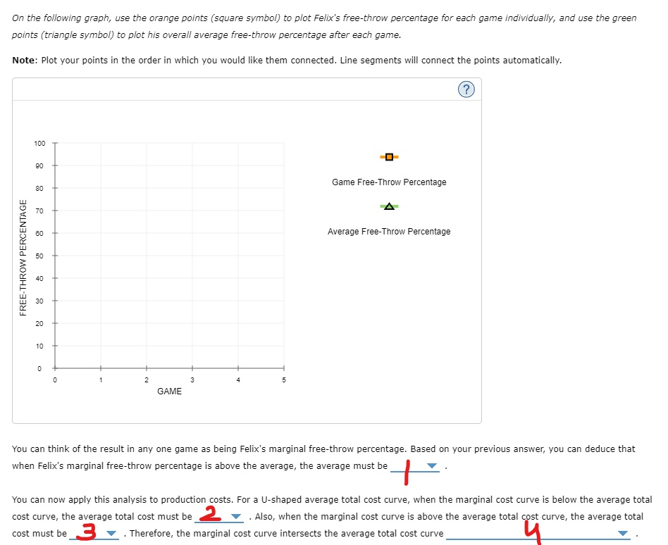
On the following graph, use the orange points (square symbol) to plot Felix's free-throw percentage for each game individually, and use the green
points (triangle symbol) to plot his overall average free-throw percentage after each game.
Note: Plot your points in the order in which you would like them connected. Line segments will connect the points automatically.
(?)
100
90
Game Free-Throw Percentage
80
70
60
Average Free-Throw Percentage
50
40
30
20
10
1
2
3
GAME
You can think of the result in any one game as being Felix's marginal free-throw percentage. Based on your previous answer, you can deduce that
when Felix's marginal free-throw percentage is above the average, the average must be
You can now apply this analysis to production costs. For a U-shaped average total cost curve, when the marginal cost curve is below the average total
cost curve, the average total cost must be 2
cost must be ▼. Therefore, the marginal cost curve intersects the average total cost curve
Also, when the marginal cost curve is above the average total cost curve, the average total
FREE-THROW PERCENTAGE

Consider the following scenario to understand the relationship between marginal and average values. Suppose Felix is a professional basketball player,
and his game log for free throws can be summarized in the following table.
Fill in the columns with Felix's free-throw percentage for each game and his overall free-throw average after each game.
Game
Game Result
Total
Game Free-Throw Percentage
Average Free-Throw Percentage
1
6/8
6/8
75
75
2
2/8
8/16
3
2/4
10/20
8/10
18/30
5
8/10
26/40
On the following graph, use the orange points (square symbol) to plot Felix's free-throw percentage for each game individually, and use the green
points (triangle symbol) to plot his overall average free-throw percentage after each game.
Note: Plot your points in the order in which you would like them connected. Line segments will connect the points automatically.
100
90
Game Free-Throw Percentage
80
70
60
Average Free-Throw Percentage
50
40
E-THROW PERCENTAGE

Expert Solution

This question has been solved!

Explore an expertly crafted, step-by-step solution for a thorough understanding of key concepts.

This is a popular solution!

SEE SOLUTION Check out a sample Q&A here

Step 1

VIEW

Step 2

VIEW

Trending now

This is a popular solution!

Step by step

Solved in 2 steps with 3 images

SEE SOLUTION Check out a sample Q&A here

Similar questions

Use the following graph to illustrate the relationship between the cost per bag of potato chips and the quantity of potato chips produced if it has a minimum point at $4 a bag and 4 bags. Put a point to show the minimum point Screenshot attached below thanks just graph what the question is asking
8. According to the Americans with Disabilities Act, the slope of a wheelchair ramp must be no greater than 1/12 (1 foot gain in height for every 12 feet of horizontal distance). What is the length of ramp needed to gain a height of 4 feet? Round your answer to the nearest tenth of a foot. The ramp is feet long.
O O O O O D c. :- 5. b. 4. a 10 3. The value of the x-intercept for the graph of 4x - 5y = 40 is %3D
Student Loans Data for selected years from 2011and projected to 2023 can be used to show that thebalance of federal direct student loans y, in billions ofdollars, is related to the number of years after 2010,x, by the function y = 130.7x + 699.7.a. Graph the function for x-values corresponding2010 to 2025.b. Find the value of y when x is 13.c. What does this function predict the balance offederal direct student loans will be in 2029?(Source: U.S. Office of Management and Budget)
Given the following, explain whether or not it is appropriate to use the graph to predict the price of a Corolla that is fourteen years old. Why or why not?
What is one property of a stationary time series? Question 23 options: The datapoints demonstrate a clear seasonal pattern The mean remains constant over time It is plotted as a straight horizontal line It demonstrates an upward trend
Graph the solution set. y > 6 O ● No Solution Help -10 -9 -8 -7 -6 -5 -4 -3 -2 -1 L 10 9 8 7 6 5 4 3 2 1 -1 -2 -3 -4 -5 -6 -7 1 -8 -9 -10 2 3 4 5 6 7 8 9 10 Clear All W Fill WebAssign. Graphing Tool Graph Layers After you add an object to the graph you can use Graph Layers to view and edit its properties.
SupposeWorldwide-Link offers an international calling plan that charges $10.00 per month plus $0.30 per minute for calls outside the United States. Requirements R1. Under this plan, what is your monthly international long-distance cost if you call Europe for a. 20 minutes? b. 50 minutes? c. 95 minutes? R2. Draw a graph illustrating your total cost under this plan. Label the axes, and show your costs at 20, 50, and 95 minutes.
Page < 1 of 2 B. x + 1 = 0 O P ZOON 16. Write an equation of the line perpendicular to the graph of x = 3 and passing through D(4, -1). A. x-4=0 C. y + 1 = 0 D. y -4 = 0