
MATLAB: An Introduction with Applications
6th Edition
ISBN: 9781119256830
Author: Amos Gilat
Publisher: John Wiley & Sons Inc
expand_more
expand_more
format_list_bulleted
Related questions
Question
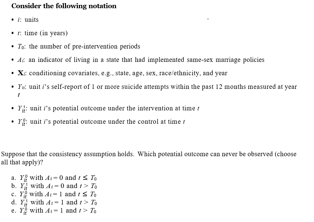

Transcribed Image Text:Consider the following notation
• i: units
•t: time (in years)
To: the number of pre-intervention periods
• A: an indicator of living in a state that had implemented same-sex marriage policies
• Xi: conditioning covariates, e.g., state, age, sex, race/ethnicity, and year
• Yit: unit i's self-report of 1 or more suicide attempts within the past 12 months measured at year
t
Y: unit i's potential outcome under the intervention at time t
Yo: unit i’s potential outcome under the control at time t
Suppose that the consistency assumption holds. Which potential outcome can never be observed (choose
all that apply)?
a. Y with Ai= 0 and t ≤ To
b. Y
with Ai = 0 and t > To
c. Y with Ai= 1 and t ≤ To
d. Y with Ai= 1 and t > To
e. Y with Ai = 1 and t > To
Expert Solution
This question has been solved!
Explore an expertly crafted, step-by-step solution for a thorough understanding of key concepts.

Step by stepSolved in 3 steps with 21 images

Knowledge Booster

Similar questions
- The times for the mile run of a large group of college male students are approximately Normal with mean µ = 7.11 minutes and standard deviation o = 0.74 minutes. Use a table of areas to answer the following: (a) What percent of these men run a mile between 7.11 minutes and 8 minutes? (b) What percent of these men run a mile in under 5 minutes? (c) What percent of these men ran the mile in over 9 minutes? (d) What percent of these men run a mile between 7 minutes to 8 minutes?arrow_forward(a) how many subjects are needed to estimate the mean number of books read the previous year with six books with 90% confidence?arrow_forwardglucose levels in oatients free of diabetes are assumed to follow a normal distribution with a mean of 120 and a standard deviation of 16. What proportion of patients have glucose levels exceesing 115?arrow_forward
- What raw score for age corresponds to a z- score of +4.50, given a mean of 12.0 years and a standard deviation of 4.0 years?arrow_forwardThe best depiction of a population characteristic is a(an): Dependent variable Statistic Independent variable Parameterarrow_forwardSuppose the mean retail price oer gallon of regular gasoline int the United States is $3.42 with a standard eviation of $0.40 and the retail price per gallon has a normal bell shaped distribution. Use the Empirical Rule to answer the following quesitona. What percentage of regular gasoline sold between $2.62 and $3.82 per gallon? what percentage of regualr gasoline sold for more the $3.82 per gallon?arrow_forward
- One important consideration in determining which location is best for a new retail business is the amount of traffic that passes the location each business day. Counters are placed at each of four locations on the five weekdays, and the number of cars passing each location is recorded in the table below. At 0.05 level of significance, is there sufficient evidence of a significant difference in the mean number of cars per day at the four locations?Using MS Excel,what is the computed value of the F statistic ? * Location II II IV 45 48 44 39 50 60 50 49 39 40 38 39 44 45 42 40 42 43 44 43 0.76 2.23 1.19 0.84arrow_forwardThe serum cholesterol levels (in 244, 235, 249, 237, 228, 220, 201, 259, 191, 198, 240, 196, 222, 252, 203, 211, 215, 254 Send data to calculator (a) mg th Find 30 and 75th percentiles for these cholesterol levels. (b) dL (If necessary, consult a list of formulas.) The 30th percentile: -) of 18 individuals are The 75th percentile: mg dL mg dLarrow_forwardThe average house has 13 paintings on its walls. Is the mean different for houses owned by teachers? The data show the results of a survey of 12 teachers who were asked how many paintings they have in their houses. Assume that the distribution of the population is normal. 12, 14, 14, 14, 15, 14, 14, 14, 12, 13, 15, 14 What can be concluded at the αα = 0.01 level of significance? For this study, we should use The null and alternative hypotheses would be: H0:H0: H1:H1: The test statistic = (please show your answer to 3 decimal places.) The p-value = (Please show your answer to 4 decimal places.) The p-value is αα Based on this, we should the null hypothesis. Thus, the final conclusion is that ... The data suggest the population mean is not significantly different from 13 at αα = 0.01, so there is sufficient evidence to conclude that the population mean number of paintings that are in teachers' houses is equal to 13. The data…arrow_forward
arrow_back_ios
arrow_forward_ios
Recommended textbooks for you
- MATLAB: An Introduction with ApplicationsStatisticsISBN:9781119256830Author:Amos GilatPublisher:John Wiley & Sons Inc
 Probability and Statistics for Engineering and th...StatisticsISBN:9781305251809Author:Jay L. DevorePublisher:Cengage Learning
 Statistics for The Behavioral Sciences (MindTap C...StatisticsISBN:9781305504912Author:Frederick J Gravetter, Larry B. WallnauPublisher:Cengage Learning
  Elementary Statistics: Picturing the World (7th E...StatisticsISBN:9780134683416Author:Ron Larson, Betsy FarberPublisher:PEARSON
 The Basic Practice of StatisticsStatisticsISBN:9781319042578Author:David S. Moore, William I. Notz, Michael A. FlignerPublisher:W. H. Freeman
 Introduction to the Practice of StatisticsStatisticsISBN:9781319013387Author:David S. Moore, George P. McCabe, Bruce A. CraigPublisher:W. H. Freeman
MATLAB: An Introduction with Applications
Statistics
ISBN:9781119256830
Author:Amos Gilat
Publisher:John Wiley & Sons Inc
Probability and Statistics for Engineering and th...
Statistics
ISBN:9781305251809
Author:Jay L. Devore
Publisher:Cengage Learning
Statistics for The Behavioral Sciences (MindTap C...
Statistics
ISBN:9781305504912
Author:Frederick J Gravetter, Larry B. Wallnau
Publisher:Cengage Learning
Elementary Statistics: Picturing the World (7th E...
Statistics
ISBN:9780134683416
Author:Ron Larson, Betsy Farber
Publisher:PEARSON
The Basic Practice of Statistics
Statistics
ISBN:9781319042578
Author:David S. Moore, William I. Notz, Michael A. Fligner
Publisher:W. H. Freeman
Introduction to the Practice of Statistics
Statistics
ISBN:9781319013387
Author:David S. Moore, George P. McCabe, Bruce A. Craig
Publisher:W. H. Freeman