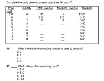
Complete the table below to answer questions 46. and 47.:PriceQuantityCost$18161412108642012345678Total RevenueMarginal RevenueMarginal$0X$2.00$16$162.5028123.003.504.004.505.005.506.00What is the profit-maximizing number of units to produce?What is the profit-maximizing price?4646.a. 2b. 4c. 6d. 847.a. $14b. $10c. $6d. $4

Remember the formulas:Total Revenue (TR) = Price (P) x quantity (Q)Marginal revenue (MR) = change in…

Answered: Complete the table below to answer…

ENGR.ECONOMIC ANALYSIS

14th Edition

ISBN:9780190931919

Author:NEWNAN

Publisher:NEWNAN

Chapter1: Making Economics Decisions

Section: Chapter Questions

Problem 1QTC

See similar textbooks

Similar questions

Sally runs a vegetable stand. The following table shows two points on the demand curve for the heirloom tomatoes she sells: Price $3.50 $2.25 Quantity demanded per week 150,000 250,000 Sally's marginal revenue from lowering the price of tomatoes from $3.50 to $2.25 is $ 0.375. (Enter your response rounded to two decimal places.) Lowering the price from $3.50 to $2.25 results in an output effect of $ and a price effect of $. (Enter your responses as whole numbers and include a minus sign if necessary.)
E2
Price, P (dollars per pound) 10 0 QUESTION 5: COST STRUCTURES Feasible set 20,000 40,000 60,000 Quantity of Cheerios, Q (pounds) ● Isoprofit curve: $60,000 ● Isoprofit curve: $34,000 Isoprofit curve: $10,000 Isoprofit curve: $0 Demand curve 80,000 The figure to the left shows the isoprofit curves and demand curve for Cheerios breakfast cereal. Draw a diagram to show how the figure would change in each of the following cases. To make sketching the curves easier, assume the demand curve is linear. In each case, can you say what would happen to the price and the profit? a) A rival company producing a similar brand slashes its prices. b) The cost of producing Apple-Cinnamon Cheerios rises to $3 per pound. c) General Mills introduces a local advertising campaign costing $10,000 per week.
Attempts 0 2. Calculating marginal revenue from a linear demand curve The blue curve on the following graph represents the demand curve facing a firm that can set its own prices. Use the graph input tool to help you answer the following questions. You will not be graded on any changes you make to this graph. Note: Once you enter a value in a white field, the graph and any corresponding amounts in each grey field will change accordingly. 160 140 120 100 A Demand 40 12 PRICE (Dollars per unit) 200 Keep the Highest 0/5 180 20 0 0 4 16 20 24 28 32 36 40 QUANTITY (Units) Graph Input Tool Market for Goods I Quanded (Units) Demand Price (Dollars per unit) 20 100.00 (?
Price and cost (dollars) 50 40 .ATC 10 MC MR 10 Quantity (thousands of households) 20 30 40 50 The above figure represents the market for cable television in Oakland, Florida. Time Warner Communications (TWC) is the sole provider of cable television to the residents of this Central Florida community. If TWC is left unregulated, what is the price of cable television in Oakland? $20 $30 $10 $40 30 20
Move the cursor to draw the marginal revenue curve using the information in the following table. Quantity Produced 0 1 2 3 4 5 6 80 70 60 50 400 30 20 10 07 Price ($) 80 75 70 65 60 55 50 2 Total Revenue ($) 0 75 140 195 240 275 300 Marginal Revenue ($) 3 4 Quantity Produced 5 6
Co Assignment Content 1) When the Price is $4 the quantity supplied of hats is 100. If the price changes to $6 dollars and the quantity supplied changes to 400, is the elasticity of supply elastic, inelastic or unit elastic? How did you reach that conclusion? 2) Why will economic profits for firms in a perfectly competitive industry tend to vanish in the long run? What about accounting AS 12
1. Price and output in a competitive price-searcher market Consider a price-searching firm, Sean's Fire Engines, which sells fire engines in the fictional country of Pyrotania. Initially, Sean's produced six fire engines but then decided to increase production to seven fire engines. The following graph shows the demand curve the firm faces. To sell the additional engine, Sean's must lower its price from $100,000 to $50,000 per engine. (Hint: Sean's Fire Engines gains revenue from the additional engine it sells, but it also loses revenue from the initial six engines because it sells them all at the lower price.) On the following graph, use the purple rectangle (diamond symbols) to shade the area representing the revenue lost from the initial six engines by selling at $50,000 rather than $100,000. Then use the green rectangle (triangle symbols) to shade the area representing the revenue gained from selling an additional engine at $50,000. re engine) 250 225 200 Q Search Revenue Lost Col
Complete the following table and identify the profit maximising and output. b. What is true about marginal revenue and marginal costs when profit is maximized. c. What would be the profit-maximizing level of output if price fell to $9?
2. The demand curve facing a competitive firm The following graph illustrates the market for small moving trucks in Bloomington, IN, during Indiana's fall move-in week. PRICE (Dollars per small truck) 100 90 Supply X 2 3 6 7 8 QUANTITY (Hundreds of small trucks) 80 70 60 50 40 30 20 10 0 Demand 0 1 4 5 9 10 ? Suppose that YouYeet is one of over a dozen competitive firms in the Bloomington area that offers moving truck rentals. Based on the preceding graph showing the weekly market demand and supply curves, the price You Yeet must take as given is $
Macmillan Learning Ⓒ The graph contains individual supply curves for the only two firms in a hypothetical market for stuffed animals. Place the market supply curve at the correct location on the graph. Then, consider what would happen to the market if a third supplier enters the market, holding all else constant. Price per Stuffed Animal ($) 10 Incorrect 8 7 6 5 4 3 2 11 0 0 Market for Stuffed Animals Firm 1 Market Firm 2 1,000 2,000 3,000 4,000 5,000 6,000 7,000 8,000 9,000 10,000 Quantity of Stuffed Animals A third firm would mean market supply increases.
Pi ce CA Per pica) 75 55 30 MR Quast (paus pe 40 The figure above shows the cost curves of a profit-maximizing perfectly competitive firm. 8) What are the characteristics of a perfectively competitive market? 9) what is the equilibrium output and price? 10) calculate the producer and consumer surplus

SEE MORE QUESTIONS

Recommended textbooks for you

ENGR.ECONOMIC ANALYSIS

Economics

ISBN:

9780190931919

Author:

NEWNAN

Publisher:

Oxford University Press

Principles of Economics (12th Edition)

Economics

ISBN:

9780134078779

Author:

Karl E. Case, Ray C. Fair, Sharon E. Oster

Publisher:

PEARSON

Engineering Economy (17th Edition)

Economics

ISBN:

9780134870069

Author:

William G. Sullivan, Elin M. Wicks, C. Patrick Koelling

Publisher:

PEARSON

ENGR.ECONOMIC ANALYSIS

Economics

ISBN:

9780190931919

Author:

NEWNAN

Publisher:

Oxford University Press

Principles of Economics (12th Edition)

Economics

ISBN:

9780134078779

Author:

Karl E. Case, Ray C. Fair, Sharon E. Oster

Publisher:

PEARSON

Engineering Economy (17th Edition)

Economics

ISBN:

9780134870069

Author:

William G. Sullivan, Elin M. Wicks, C. Patrick Koelling

Publisher:

PEARSON

Principles of Economics (MindTap Course List)

Economics

ISBN:

9781305585126

Author:

N. Gregory Mankiw

Publisher:

Cengage Learning

Managerial Economics: A Problem Solving Approach

Economics

ISBN:

9781337106665

Author:

Luke M. Froeb, Brian T. McCann, Michael R. Ward, Mike Shor

Publisher:

Cengage Learning

Managerial Economics & Business Strategy (Mcgraw-…

Economics

ISBN:

9781259290619

Author:

Michael Baye, Jeff Prince

Publisher:

McGraw-Hill Education

SEE MORE TEXTBOOKS