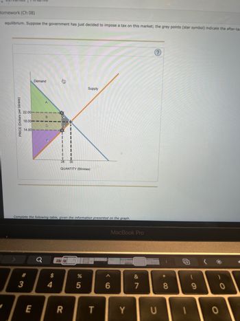
## Government-Imposed Tax on Market Equilibrium### Graph Analysis of After-Tax Market EquilibriumThis graph depicts the effects of a government-imposed tax on a market, showing the shifts in supply and demand curves. The labeled points and areas represent critical components of the market dynamics:1. **Axes**: - The vertical axis represents the **Price (Dollars per blinkie)**. - The horizontal axis represents the **Quantity (Blinkies)**.2. **Curves**: - The **Demand** curve slopes downward from left to right, indicating that as the price decreases, the quantity demanded increases. - The **Supply** curve slopes upward from left to right, indicating that as the price increases, the quantity supplied increases.3. **Equilibrium Points**: - The **pre-tax equilibrium** is where the original supply and demand curves intersect. - The **after-tax equilibrium** points are indicated by grey star symbols. These denote the new intersection points of the supply and demand curves after a tax has been placed on the market.4. **Price Changes**: - **Pre-tax Equilibrium Price**: This original intersection sets the price and quantity without any tax intervention. - **Post-tax Price to Buyers** is reflected at point B (about $22.00). - **Post-tax Price to Sellers** is reflected at point E (about $14.00). 5. **Quantity Changes**: - **Pre-tax Quantity** is at the initial intersection of supply and demand curves. - **Post-tax Quantity** decreases to the new equilibrium (about 28 units).6. **Areas**: - **A and F (Consumer and Producer Surplus Lost)**: These areas may represent the deadweight loss due to the tax, which is the loss of total surplus that results from the tax. - **B and D (Consumer and Producer Surplus with Tax)**: These areas indicate the remaining consumer and producer surplus after the tax. - **C (Tax Revenue)**: This area represents the government's tax revenue derived from the tax imposed on each unit sold.### Instructions:Complete the following table using the information extracted and interpreted from the graph.---This detailed analysis should help students understand the impact of government-imposed taxes on market equilibrium, highlighting the shifts and changes in price, quantity, and welfare within the market. 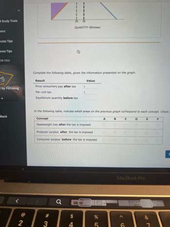### Understanding the Impact of Taxation on Market Equilibrium#### IntroductionThis section aims to help students understand the changes in market equilibrium and welfare distribution due to the imposition of a tax, using graphical representation and data tables.---#### Graph ExplanationThe provided graph depicts the market for "Blinkies" with the quantity on the x-axis and price on the y-axis. Key points illustrated are:- **Equilibrium Quantity Before Tax:** Initially, the market equilibrium quantity is shown at 36 units of Blinkies.- **Quantity Change After Tax:** With the imposition of tax, the quantity decreases to 28 units.The graph illustrates areas representing various economic concepts such as consumer surplus, producer surplus, and deadweight loss.---#### Data Table CompletionStudents should use the graph to fill in the following table:**Results Table**| Result | Value ||---------------------------------------|-------------------------|| Price consumers pay after tax | \_\_\_\_\_\_\_\_\_\_\_ || Per-unit tax | \_\_\_\_\_\_\_\_\_\_\_ || Equilibrium quantity before tax | \_\_\_\_\_\_\_\_\_\_\_ |---#### Economic Impact AnalysisIn the subsequent table, match the correct areas on the graph to the relevant economic concept based on their locations and shapes on the graph.**Concept Identification Table**| Concept | A | B | C | D | E | F ||----------------------------------------------|------|------|------|------|------|------|| Deadweight loss after the tax is imposed | ☐ | ☐ | ☐ | ☐ | ☐ | ☐ || Producer surplus after the tax is imposed | ☐ | ☐ | ☐ | ☐ | ☐ | ☐ || Consumer surplus before the tax is imposed | ☐ | ☐ | ☐ | ☐ | ☐ | ☐ |---#### Detailed Concept Explanation- **Deadweight Loss After Tax:** Represents the lost welfare because taxes create a gap between the price consumers pay and the price producers receive, leading to a reduction in the traded quantity.- **Producer Surplus After Tax:** The difference between what producers are willing to accept and what they actually receive after the tax is imposed.- **

Consumer surplus is the area above the market price and below the demand curve upto quantity…

Complete the following table, given the information presented on the graph. Result Price consumers pay after tax Per-unit tax Equilibrium quantity before tax $ 999 Value In the following table, indicate which areas on the previous graph correspond to each concept. Check Concept Deadweight loss after the tax is imposed Producer surplus after the tax is imposed Consumer surplus before the tax is imposed A 00 C 0 D E 00 MacBook Pro F 000 C

Complete the following table, given the information presented on the graph. Result Price consumers pay after tax Per-unit tax Equilibrium quantity before tax $ 999 Value In the following table, indicate which areas on the previous graph correspond to each concept. Check Concept Deadweight loss after the tax is imposed Producer surplus after the tax is imposed Consumer surplus before the tax is imposed A 00 C 0 D E 00 MacBook Pro F 000 C

ENGR.ECONOMIC ANALYSIS

14th Edition

ISBN:9780190931919

Author:NEWNAN

Publisher:NEWNAN

Chapter1: Making Economics Decisions

Section: Chapter Questions

Problem 1QTC

See similar textbooks

Similar questions

CHECK OUT IMAGE PLS
Calculate the consumer surplus Calculate the producer surplus before the tax
The following graph represents the demand and supply for blinkies (an imaginary product). The black point (plus symbol) indicates the pre-tax equilibrium. Suppose the government has just decided to impose a tax on this market; the grey points (star symbol) indicate the after-tax scenario. PRICE (Dollars per blinkie) Demand 42.00---== 36.00 30.00 B II Supply QUANTITY (Blinkies)
Suppose that the government imposes a per-unit tax on cell phones. The tax is imposed on producers of cell phones and the amount of the tax is $50 per cell phone. The following graph shows the effect of the tax. Use the graph to answer the following questions. a) How much of the tax per cell phone is paid by producers? How much of the tax per cell phone is paid by consumers? b) How much tax revenue (in total) does the government collect from the tax imposed on cell phones? c) What is the amount of the deadweight loss due to the presence of the tax on cell phones?
PRICE (Dollars per handbag) 500 450 400 350 300 250 200 150 100 50 0 0 Demand Tax Wedge 160 320 480 640 800 960 1120 1280 1440 1600 QUANTITY (Handbags) Consumer Surplus Producer Surplus After Tax Tax Revenue + Supply Deadweight Loss Before Tax (Dollars) Complete the following table by using the previous graphs to determine the values of consumer and producer surplus before the tax, and consumer surplus, producer surplus, tax revenue, and deadweight loss after the tax. Note: You can determine the areas of different portions of the graph by selecting the relevant area. 0 0 Tax Revenue After Tax (Dollars) A Consumer Surplus Producer Surplus Deadweight Loss Note:- Do not provide handwritten solution. Maintain accuracy and quality in your answer. Take care of plagiarism. Answer completely. You will get up vote for sure.
A5
On the following graph, use the black curve (plus symbols) to illustrate the deadweight loss in these cases. (Hint: Remember that the area of a triangle is equal to x Base × Height. In the case of a deadweight loss triangle found on the graph input tool, the base is the amount of the tax and the height is the reduction in quantity caused by the tax.) 2400 2160 1920 Deadweight Loss 1680 1440 1200 960 720 480 240 10 20 30 40 50 60 70 80 90 100 TAX (Dollars per bottle) As the tax per bottle increases, deadweight loss DEADWEIGHT LOSS (Dollars)
Please assist with the following questions 1. Calculate the (i) consumer surplus BREFORE THE TAX (ii) producers surplus BEFORE THE TAX 2. For the market of cigarettes WITH THE TAX please indicate (i) the tax (ii) price paid by consumers (iii) price received by producers (iv) Quantitiy of cigarettes sold thank you
The following graph represents the demand and supply for pinckneys (an imaginary product). The black point (plus symbol) indicates the pre-tax equilibrium. Suppose the government has just decided to impose a tax on this market; the grey points (star symbol) indicate the after-tax scenario. Demand Supply A 16, 18 21.00 18.00- D E 15.00 F 12 16 QUANTITY (Pinckneys) PRICE (Dollars per pinckney)
I need help with a few calculations if possible please? Calculate the producer surplus before the tax. Calculate the consumer surplus after the tax. Calculate the producer surplus after the tax. Tax revenue Deadweight loss Total surplus after tax
Doyle and Samphantharak (2008) find that when a 5% gas tax is implemented, prices consumers pay for gas increase by about 4%. What role does demand elasticity play in determining the size of this price change? That is, under what demand elasticity cases would the price change be closer to 5%, or closer to 0%? Illustrate and explain using supply-and-demand graph(s)..
The accompanying graph depicts a hypothetical market for salt. Suppose that an excise or commodity tax is levied on consumers in an attempt to curb blood pressure problems. Show the effect of the tax by shifting the appropriate curve(s). Macmillan Learning Who has the larger tax burden? Consumers (buyers) Producers (suppliers) The tax burdens are equal Why is the tax burden as you described in in the question above? Consumers are the ones paying the tax. Demand is less elastic than supply. Both supply and demand are perfectly elastic. Supply is less elastic than demand. Demand is more elastic than supply. Price (S/kilogram) 9 3 Market for Salt D 4 5 Quantity (in kilograms). S 10