
MATLAB: An Introduction with Applications
6th Edition
ISBN: 9781119256830
Author: Amos Gilat
Publisher: John Wiley & Sons Inc
expand_more
expand_more
format_list_bulleted
Related questions
Question
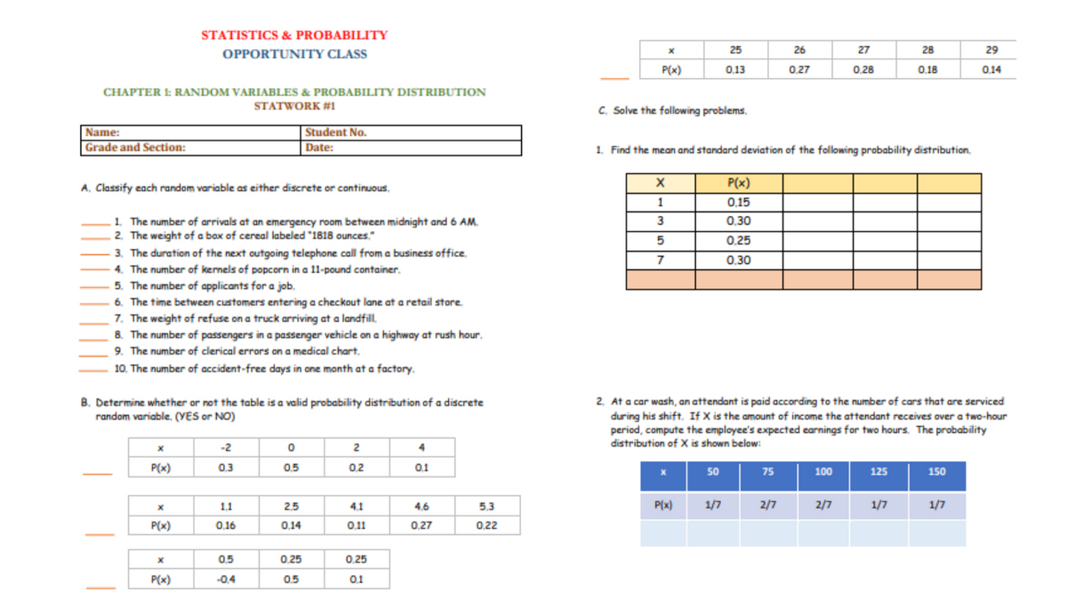

Transcribed Image Text:STATISTICS & PROBABILITY
OPPORTUNITY CLASS
25
26
27
28
29
P(x)
0,13
0,27
0,28
0,18
0.14
CHAPTER 1: RANDOM VARIABLES & PROBABILITY DISTRIBUTION
STATWORK #1
C. Solve the following problems.
Name:
Student No.
Grade and Section:
Date:
1. Find the mean and standard deviation of the following probability distribution.
A, Classify each random variable as either discrete or continuous,
P(x)
1
0.15
1. The number of arrivals at an emergency room between midnight and 6 AM.
2. The weight of a box of cereal labeled "1818 ounces."
0.30
5
0.25
3. The duration of the next outgoing telephone call from a business office.
4. The number of kernels of popcorn in a 11-pound container.
5. The number of applicants for a job.
6. The time between customers entering a checkout lane at a retail store.
7. The weight of refuse on a truck arriving at a landfill,
8. The number of passengers in a passenger vehicle on a highway at rush hour,
9. The number of clerical errors on a medical chart.
7
0.30
10. The number of accident-free days in one month at a factory.
2. At a car wash, an attendant is paid according to the number of cars that are serviced
during his shift. If X is the amount of income the attendant receives aver a two-hour
period, compute the employee's expected earnings for two hours. The probability
distribution of X is shown below:
B. Determine whether or not the table is a valid probability distribution of a discrete
random variable, (VES or NO)
-2
2
4
P(x)
0.3
0.5
0.2
0.1
50
75
100
125
150
1,1
25
4,1
4.6
5.3
P(x)
1/7
2/7
2/7
1/7
1/7
P(x)
0,16
0,14
011
0.27
0,22
0.5
0,25
0,25
P(x)
-0.4
0.5
0.1
|

Transcribed Image Text:3. A woman can earn 50,000 pesos in one year with a probability of 0.35 or lose 15,000 over
the same period with a probability of 0,65 by investing in the stocks of a certain
company, Compute her expected earnings from this investment.
(Amount of Gains and Loses)
P(z)
4. A company estimates that about 0,7% of their products will fail after the 1-year
warranty but within two years from the date of purchase, If this happens, the company
will pay a replacement cost Php3,500, If the company offers its customers an extended
warranty covering a period of two years for the price of Php 480, what is the company's
expected value for each extended warranty that it can sell?
(Amount of Gains and Loses)
P(z)
Expert Solution
This question has been solved!
Explore an expertly crafted, step-by-step solution for a thorough understanding of key concepts.

This is a popular solution

Trending nowThis is a popular solution!

Step by stepSolved in 2 steps

Knowledge Booster

Similar questions
- • A) Given the data Pulse Rate (beats per minute) Mean St. Dev. Distribution Males 69.6 11.3 Normal Females 74.0 12.5 Normal a. Find the probability that a female has a pulse rate less than 60 beats per minute. b. Find the probability that a male has a pulse rate grater than 80 beats per minute. c. Find the probability that a m ale has a pulse rate between 65 beats per minute and 85 beats per minute. • B) Snow White. Disney World required that women employed as a Snow White character must have a height between 64 in and 67 in o Find the percentage of women meeting the height requirement o If the height requirements are changed to exclude the shortest 40% of women and the tallest 5% of women, what are the new height requirements?arrow_forwardDetermine whether the value is a discrete random variable, continuous random variable, or not a random variable. a. The time required to download a file from the Internet b. The height of a randomly selected giraffe c. The eye color of people on commercial aircraft flights d. The number of free-throw attempts before the first shot is made e. The amount of rain in City B during April f. The number of hits to a website in a day a. Is the time required to download a file from the Internet a discrete random variable, a continuous random variable, or not a random variable? A. It is a discrete random variable. B. It is a continuous random variable. C. It is not a random variable. b. Is the height of a randomly selected giraffe a discrete random variable, a continuous random variable, or not a random variable? A. It is a discrete random variable. B. It is a continuous random variable. C. It is not a random variable c. Is the eye color of people on commercial aircraft flights a discrete random…arrow_forwardThe Census Bureau gives this distribution for the number of people in American households in 2016. Family size 1 2 4 6. 7 Proportion 0.28 0.35 0.15 0.13 0.06 0.02 0.01 Note: In this table, 7 actually represents households of size 7 or greater. But for purposes of this exercise, assume that it means only households of size exactly 7. Suppose you take a random sample of 4000 American households. About how many of these households will be of size 2? Sizes 3 to 7? The number of households of size 2 is about The number of households of size 3 to 7 is aboutarrow_forward
- Four coins are tossed, and the number of heads is recorded. Shade the region on the histogram that gives the indicated probability. P(x > 2) Which of the following shaded regions gives the indicated probability? (Type A, B, C, or D.) A) 0.5- 0.38- 0.25- 0.13- 0- 0.5- 0.38 0.25- 0.13- लट 0 1 2 3 4 01 2 3 4 B) D) 0.5- 0.38- 0.25- 0.13- 0- 0.5- 0.38 0.25 0.13- 0- 0 1 2 3 4 0 1 2 3 4arrow_forwardDetermine whether the value is a discrete random variable, continuous random variable, or not a random variable. a. The time required to download a file from the Internet b. The number of fish caught during a fishing tournament c. The response to the survey question "Did you smoke in the last week?" d. The distance a baseball travels in the air after being hit e. The number of hits to a website in a day f. The time it takes for a light bulb to burn out a. Is the time required to download a file from the Internet a discrete random variable, a continuous random variable, or not a random variable? C O A. It is a continuous random variable. O B. It is a discrete random variable. O C. It is not a random variable. b. Is the number of fish caught during a fishing tournament discrete random variable, a continuous random variable, or not a random variable? O A. It is a continuous random variable. O B. It is a discrete random variable. O C. It is not a random variable c. Is the response to the…arrow_forwardThe probability is 0.4 that a traffic fatality involves an intoxicated or alcohol-impaired driver or nonoccupant. In six traffic fatalities, find the probability that the number, Y, which involve an intoxicated or alcohol-impaired driver or nonoccupant is a. exactly three; at least three; at most three. b. between two and four, inclusive. c. Find and interpret the mean of the random variable Y. a. The probability that exactly three traffic fatalities involve an intoxicated or alcohol-impaired driver or nonoccupant is nothing. (Round to four decimal places as needed.) The probability that at least three traffic fatalities involve an intoxicated or alcohol-impaired driver or nonoccupant is nothing. (Round to four decimal places as needed.) The probability that at most three traffic fatalities involve an intoxicated or alcohol-impaired driver or nonoccupant is nothing. (Round to four decimal places as needed.) b. The probability that between two and four…arrow_forward
arrow_back_ios
arrow_forward_ios
Recommended textbooks for you
- MATLAB: An Introduction with ApplicationsStatisticsISBN:9781119256830Author:Amos GilatPublisher:John Wiley & Sons Inc
 Probability and Statistics for Engineering and th...StatisticsISBN:9781305251809Author:Jay L. DevorePublisher:Cengage Learning
 Statistics for The Behavioral Sciences (MindTap C...StatisticsISBN:9781305504912Author:Frederick J Gravetter, Larry B. WallnauPublisher:Cengage Learning
  Elementary Statistics: Picturing the World (7th E...StatisticsISBN:9780134683416Author:Ron Larson, Betsy FarberPublisher:PEARSON
 The Basic Practice of StatisticsStatisticsISBN:9781319042578Author:David S. Moore, William I. Notz, Michael A. FlignerPublisher:W. H. Freeman
 Introduction to the Practice of StatisticsStatisticsISBN:9781319013387Author:David S. Moore, George P. McCabe, Bruce A. CraigPublisher:W. H. Freeman
MATLAB: An Introduction with Applications
Statistics
ISBN:9781119256830
Author:Amos Gilat
Publisher:John Wiley & Sons Inc
Probability and Statistics for Engineering and th...
Statistics
ISBN:9781305251809
Author:Jay L. Devore
Publisher:Cengage Learning
Statistics for The Behavioral Sciences (MindTap C...
Statistics
ISBN:9781305504912
Author:Frederick J Gravetter, Larry B. Wallnau
Publisher:Cengage Learning
Elementary Statistics: Picturing the World (7th E...
Statistics
ISBN:9780134683416
Author:Ron Larson, Betsy Farber
Publisher:PEARSON
The Basic Practice of Statistics
Statistics
ISBN:9781319042578
Author:David S. Moore, William I. Notz, Michael A. Fligner
Publisher:W. H. Freeman
Introduction to the Practice of Statistics
Statistics
ISBN:9781319013387
Author:David S. Moore, George P. McCabe, Bruce A. Craig
Publisher:W. H. Freeman