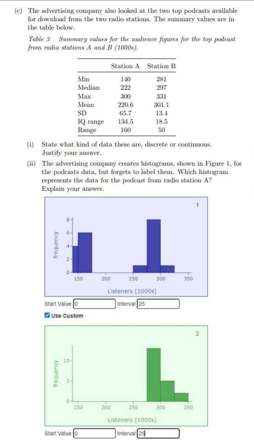
(c) The advertising company also looked at the two top podcasts availablefor download from the two radio stations. The summary values are inthe table below.Table 3 Summary values for the audience figures for the top podcastfrom radio stations A and B (1000s).frequencyMinMedianMaxMeanSDIQ rangeRange(i) State what kind of data these are, discrete or continuous.Justify your answer.(ii) The advertising company creates histograms, shown in Figure 1, forthe podcasts data, but forgets to label them. Which histogramrepresents the data for the podcast from radio station A?Explain your answer.Start Value 0Abuanbay150Use Custom10-150Start Value 0Station A Station B.140222200300220.665.7134.5160200281297331301.113.418.550250Listeners (1000s)Interval 25250300350L300Listeners (1000s)Interval 253502 An advertising company is comparing published listening figures for differentradio stations and podcasts in order to decide where is the best place to puttheir adverts. The audience figures for the last 20 quarters of radio stationsA and B are in Table 1.Table 1 Audience figures in 100 000s of radio stations A and B forthe last 20 quarters.Radio Station A Radio Station B11210610811311110910811211511511811411611511310310710510310698101100991009910098969798878892989996102104100

(c) The advertising company also looked at the two top podcasts available for download from the two radio stations. The summary values are in the table below. Table 3 Summary values for the audience figures for the top podcast from radio stations A and B (1000s). Min Median Max Mean SD IQ range Range frequency (i) State what kind of data these are, discrete or continuous. Justify your answer. (ii) The advertising company creates histograms, shown in Figure 1, for the podcasts data, but forgets to label them. Which histogram represents the data for the podcast from radio station A? Explain your answer. 150 Start Value 0 10- Use Custom Station A Station B 140 222 300 220.6 65.7 134.5 160 200 281 297 331 301.1 13.4 18.5 50 250 300 Listeners (1000s) Interval 25 350 2

(c) The advertising company also looked at the two top podcasts available for download from the two radio stations. The summary values are in the table below. Table 3 Summary values for the audience figures for the top podcast from radio stations A and B (1000s). Min Median Max Mean SD IQ range Range frequency (i) State what kind of data these are, discrete or continuous. Justify your answer. (ii) The advertising company creates histograms, shown in Figure 1, for the podcasts data, but forgets to label them. Which histogram represents the data for the podcast from radio station A? Explain your answer. 150 Start Value 0 10- Use Custom Station A Station B 140 222 300 220.6 65.7 134.5 160 200 281 297 331 301.1 13.4 18.5 50 250 300 Listeners (1000s) Interval 25 350 2

MATLAB: An Introduction with Applications

6th Edition

ISBN:9781119256830

Author:Amos Gilat

Publisher:Amos Gilat

Chapter1: Starting With Matlab

Section: Chapter Questions

Problem 1P

See similar textbooks

Similar questions

tion 2 of 15 Last summer, the Smith family drove through seven different states and visited various popular landmarks. The prices of gasoline in dollars per gallon varied from state to state and are listed below. $2.34, $2.75, $2.48, $3.58, $2.87, $2.53, $3.31 Click to download the data in your preferred format. CrunchIt! CSV Excel JMP Mac Text Minitab PC Text R SPSS TI Calc Calculate the range of the price of gas. Give your solution to the nearest cent. range: dollars per gallon DELL & 4. 7 8.
Can this be converted into a frequency histogram?
why do you think the data presented this way?
A graph that uses vertical bars to represent qualitative data is called a
The entirety of the data set will be in the two pictures
Which of the following is NOT an appropriate display for the variable of Grade Point Average? Group of answer choices Dot Plot Scatterplot Boxplot Stem and Leaf Plot Histogram
A theater company asked Its members to bring in canned food for a food drive. Use the categorlcal data to complete the frequency table. Cans Donated to Food Drive Cans Frequency soup com peas peas soup peas com corn corn peas corn peas soup soup soup peas peas peas soup soup soup com corn
The ages (in years)and heights (in inches) of all pitchers for a baseball team are listed. Find the cofficient of a variation for each of the two data sets. Then compare the result.
Answer d & e only
What is the equation of finding an estimate on a negative scatter plot?
dear sir mam how do u create a steam and leaf data plot
A national park conducts a study on the behaviour of their leopards. A few of the park's leopards are registered and receive a GPS device which allows measuring the position of the leopard. Use this example to describe the following concepts: population, sample, observation, value, and variable.