
MATLAB: An Introduction with Applications
6th Edition
ISBN: 9781119256830
Author: Amos Gilat
Publisher: John Wiley & Sons Inc
expand_more
expand_more
format_list_bulleted
Related questions
Concept explainers
Question
Exercise 3.3 Airlines Y = Delay (minutes), X = Outsource (% maintenance outsourced)
(a) Plot the data. Explain whether you expect Hawaiian to be influential.
(c) What is the predicted value at X=74.1 for both lines.
(d) State your conclusion.
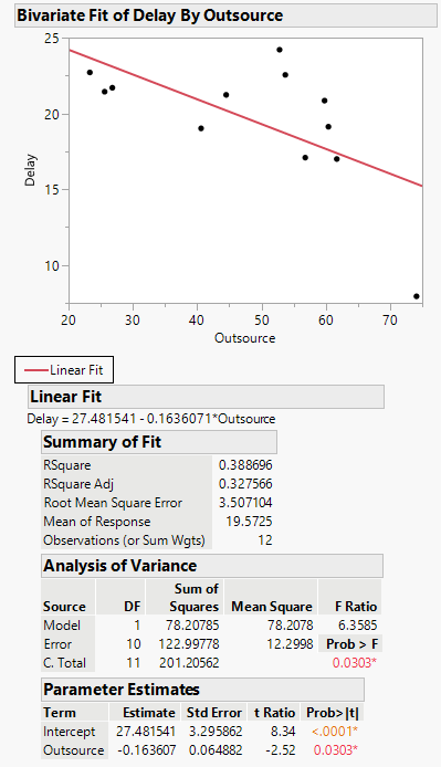

Transcribed Image Text:Bivariate Fit of Delay By Outsource
25
20
15
10
20
30
40
50
60
70
Outsource
-Linear Fit
Linear Fit
Delay = 27.481541 -0.1636071*Outsource
Summary of Fit
RSquare
RSquare Adj
Root Mean Square Error
Mean of Response
Observations (or Sum Wgts)
0.388696
0.327566
3.507104
19.5725
12
Analysis of Variance
Sum of
Squares Mean Square
78.20785
Source
DF
FRatio
Model
1
78.2078
6.3585
Error
10 122.99778
12.2998 Prob > F
C. Total
11 201.20562
0.0303*
Parameter Estimates
Term
Estimate Std Error t Ratio Prob>|t|
Intercept
27.481541 3.295862
8.34 <.0001*
Outsource -0.163607 0.064882
-2.52
0.0303*
Delay

Transcribed Image Text:Bivariate Fit of Delay By Outsource
24
22
20
18
16
20
30
40
50
60
Outsource
-Linear Fit
Linear Fit
Delay = 23.793321 - 0.0687679*Outsource
Summary of Fit
RSquare
RSquare Adj
Root Mean Square Error
Mean of Response
Observations (or Sum Wgts)
0.193961
0.10440
2.190764
20.63
11
Analysis of Variance
Sum of
Squares Mean Square
1 10.394193
9 43.195007
Source
DF
FRatio
Model
10.3942
2.1657
Error
4.7994 Prob > F
C. Total
10 53.589200
0.1752
Parameter Estimates
Term
Estimate Std Error t Ratio Prob>|t|
Intercept
23.793321 2.248731
10.58 <.0001*
Outsource -0.068768 0.046729
-1.47
0.1752
Delay
Expert Solution
This question has been solved!
Explore an expertly crafted, step-by-step solution for a thorough understanding of key concepts.

Step by stepSolved in 4 steps with 1 images

Knowledge Booster


Learn more about
Need a deep-dive on the concept behind this application? Look no further. Learn more about this topic, statistics and related others by exploring similar questions and additional content below.Similar questions
- I’m taking a probability and statistics class please get this correct because I’ve gotten wrong answers beforearrow_forwardThe correlation between hours of sleep and hours of study is r = 0.14. (a) Calculate r². (Round your answer to four decimal places.) ,2 = = (b) Choose a sentence that interprets value r². 1.96% of the variation in hours of sleep is not explained by hours of study. Variation in hours of study explains about 1.96% of the observed variation in hours of sleep. 1.96% of the variation in hours of sleep is not explained by the variation in hours of study. Hours of study explains about 1.96% of the observed variation in hours of sleep.arrow_forwardUse the estimate yest=3.3x2 - 9.4x - 0.1 to calculate a set of residuals, using a formula or a calculator. Explain your steps, then create a residual plot using this new model and assess its validityarrow_forward
- The multiple regression describes how the mean value of y is related to the xi independent variables. The parameters ?i are used to describe how the mean value of y changes for a one-unit increase in xi when the other variables are held constant. The given estimated regression equation follows where x1 is the high-school grade point average, x2 is the SAT mathematics score, and y is the final college grade point average. ŷ = −1.38 + 0.0232x1 + 0.00482x2 If the variable x2 is held constant, then only changes in x1 will impact the predicted values of ŷ. Since the coefficient of x1 is positive, for each one-unit increase of x1, the values of ŷ will increase by the value of ?1, where ?1 = . In context, for each one point increase of the high-school grade point average, the final college grade point average will increase by this amount when the SAT mathematics score does not change. If the variable x1 is held constant, then only changes in x2 will impact the predicted values of ŷ. Since the…arrow_forwardSuppose the correlation between height and weight for adults is +0.40.What proportion (or percent) of the variability in weight can be explained by the relationship with height?arrow_forwardI need in one hour pls help thankyouarrow_forward
- Below is the actual data on the speed a person walks or runs in miles/hour and the calories the person burns per lap. Find the linear equation of best fit for this data. Compare the model to the data. Does the model seem to fit the data? Explain. What is the significance of the y-intercept? What is the slope and what does it mean? What is the x-intercept and what does it mean? What is the correlation coefficient and what does it mean? Speed (mph) Calories/lap 1 42 2 31 3 27 4 41 5 40 6 40 7 39 8 38 r answers to the nearest hundredth. The y-intercept means that if a person runs at ----------mph they will burn__________ per lap. The slope means that for each mph you increase your speed, you will burn an additional------------calories pay laparrow_forwardWrite the linear model to test the hypothesis that there is no treatment effect. Clearly describe each term in the model, and the range of the subscripts. Write the null hypothesis that you are testing. Call: lm(formula = score ~ list, data = hearing) Residuals: Min 1Q Median 3Q Max -14.7500 -5.5833 -0.2083 6.3333 16.4167 Coefficients: Estimate Std. Error t value Pr(>|t|) (Intercept) 32.750 1.612 20.315 < 2e-16 *** listList2 -3.083 2.280 -1.352 0.17955 listList3 -7.500 2.280 -3.290 0.00142 ** listList4 -7.167 2.280 -3.144 0.00225 ** --- Signif. codes: 0 ‘***’ 0.001 ‘**’ 0.01 ‘*’ 0.05 ‘.’ 0.1 ‘ ’ 1 Residual standard error: 7.898 on 92 degrees of freedom Multiple R-squared: 0.1382, Adjusted R-squared: 0.1101 F-statistic: 4.919 on 3 and 92 DF, p-value: 0.00325arrow_forwardI just need the d sectionarrow_forward
arrow_back_ios
arrow_forward_ios
Recommended textbooks for you
- MATLAB: An Introduction with ApplicationsStatisticsISBN:9781119256830Author:Amos GilatPublisher:John Wiley & Sons Inc
 Probability and Statistics for Engineering and th...StatisticsISBN:9781305251809Author:Jay L. DevorePublisher:Cengage Learning
 Statistics for The Behavioral Sciences (MindTap C...StatisticsISBN:9781305504912Author:Frederick J Gravetter, Larry B. WallnauPublisher:Cengage Learning
  Elementary Statistics: Picturing the World (7th E...StatisticsISBN:9780134683416Author:Ron Larson, Betsy FarberPublisher:PEARSON
 The Basic Practice of StatisticsStatisticsISBN:9781319042578Author:David S. Moore, William I. Notz, Michael A. FlignerPublisher:W. H. Freeman
 Introduction to the Practice of StatisticsStatisticsISBN:9781319013387Author:David S. Moore, George P. McCabe, Bruce A. CraigPublisher:W. H. Freeman
MATLAB: An Introduction with Applications
Statistics
ISBN:9781119256830
Author:Amos Gilat
Publisher:John Wiley & Sons Inc
Probability and Statistics for Engineering and th...
Statistics
ISBN:9781305251809
Author:Jay L. Devore
Publisher:Cengage Learning
Statistics for The Behavioral Sciences (MindTap C...
Statistics
ISBN:9781305504912
Author:Frederick J Gravetter, Larry B. Wallnau
Publisher:Cengage Learning
Elementary Statistics: Picturing the World (7th E...
Statistics
ISBN:9780134683416
Author:Ron Larson, Betsy Farber
Publisher:PEARSON
The Basic Practice of Statistics
Statistics
ISBN:9781319042578
Author:David S. Moore, William I. Notz, Michael A. Fligner
Publisher:W. H. Freeman
Introduction to the Practice of Statistics
Statistics
ISBN:9781319013387
Author:David S. Moore, George P. McCabe, Bruce A. Craig
Publisher:W. H. Freeman