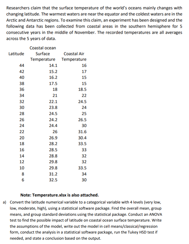
Researchers claim that the surface temperature of the world's oceans mainly changes with changing latitude. The warmest waters are near the equator and the coldest waters are in the Arctic and Antarctic regions. To examine this claim, an experiment has been designed and the following data has been collected from coastal areas in the southern hemisphere for 5 consecutive years in the middle of November. The recorded temperatures are all averages across the 5 years of data. Coastal ocean Surface Temperature Latitude 44 42 40 38 36 34 32 30 28 26 24 22 20 18 16 14 12 10 8 6 14.1 15.2 16.2 17.5 18 21 22.1 23.8 24.5 24.2 24.4 26 26.9 28.2 28.5 28.8 29.8 29.8 31.2 32.5 Coastal Air Temperature 16 17 15 15 18.5 22 24.5 24 25 26.5 30 31.6 30.4 33.5 33 32 32 33.5 34 30 Note: Temperature.xlsx is also attached. a) Convert the latitude numerical variable to a categorical variable with 4 levels (very low, low, moderate, high), using a statistical software package. Find the overall mean, group means, and group standard deviations using the statistical package. Conduct an ANOVA test to find the possible impact of latitude on coastal ocean surface temperature. Write the assumptions of the model, write out the model in cell means/classical/regression form, conduct the analysis in a statistical software package, run the Tukey HSD test if needed, and state a conclusion based on the output.

please answer 4 and 5

A medical doctor is interested in determining whether mean body temperatures are different in the morning and at night. Five patients were recruited and their body temperatures were measured first at 8 AM and then again at 10 PM. The data is in the following table: Patient 1 2 4 Morning Night 98.0 97.6 97.2 97.0 98.0 97.0 98.8 97.6 97.7 98.8 For this matched pairs experiment, you should take the differences by calculating: Morning - Night. Also, you may use the fact that the sample standard deviation of 44/V5 the differences is 0.844 and that 0.844 0.3774. What is the test statistic for the test? Round your final answer to two decimals. Next Page Page 5 of 15 126 53 1. NOV 18

A medical doctor is interested in determining whether mean body temperatures are different in the morning and at night. Five patients were recruited and their body temperatures were measured first at 8 AM and then again at 10 PM. The data is in the following table: Patient 1 3 14 5 Morning 98.0 97.6 97.2 97.0 98.0 Night 97.0 98.8 97.6 97.7 98.8 For this matched pairs experiment, you should take the differences by calculating: Morning Night. What is the alternative hypothesis of interest? OH1 : HD 0 O H1 : µp # 0 Next Page Page 4 of 15 126 NOV 18 MacBook Pro

The Focus Problem at the beginning of this chapter asks you to use a sign test with a 10% level of significance to test the claim that the overall temperature distribution of Madison, Wisconsin, is different (either way) from that of Juneau, Alaska. The monthly average data (in °F) are as follows. Month Jan. Feb. March April May June Madison 17.8 21.4 31.8 46.9 57.1 67.8 Juneau 22.8 27.5 31.8 38.6 46.2 52.7 Month July Aug. Sept. Oct. Nov. Dec. Madison 71.9 69.5 60.8 51.7 35.6 22.2 Juneau 55.6 54.9 49.3 41.1 32.5 26.3 (a) What is the level of significance? (b) Compute the sample test statistic. (Use 2 decimal places.) (c) Find the P-value of the sample test statistic

Listed below are pulse rates (beats per minute) from samples of adult males and females. Find the mean and median for each of the two samples and then compare the two sets of results. Does there appear to be a difference? Male: Female: 56 52 58 62 70 91 89 92 95 66 76 61 67 86 68 59 61 58 60 65 57 57 86 90 81 79 88 89 75 83 Find the means. The mean for males is beats per minute and the mean for females is beats per minute. (Type integers or decimals rounded to one decimal place as needed.)