
MATLAB: An Introduction with Applications
6th Edition
ISBN: 9781119256830
Author: Amos Gilat
Publisher: John Wiley & Sons Inc
expand_more
expand_more
format_list_bulleted
Related questions
Question
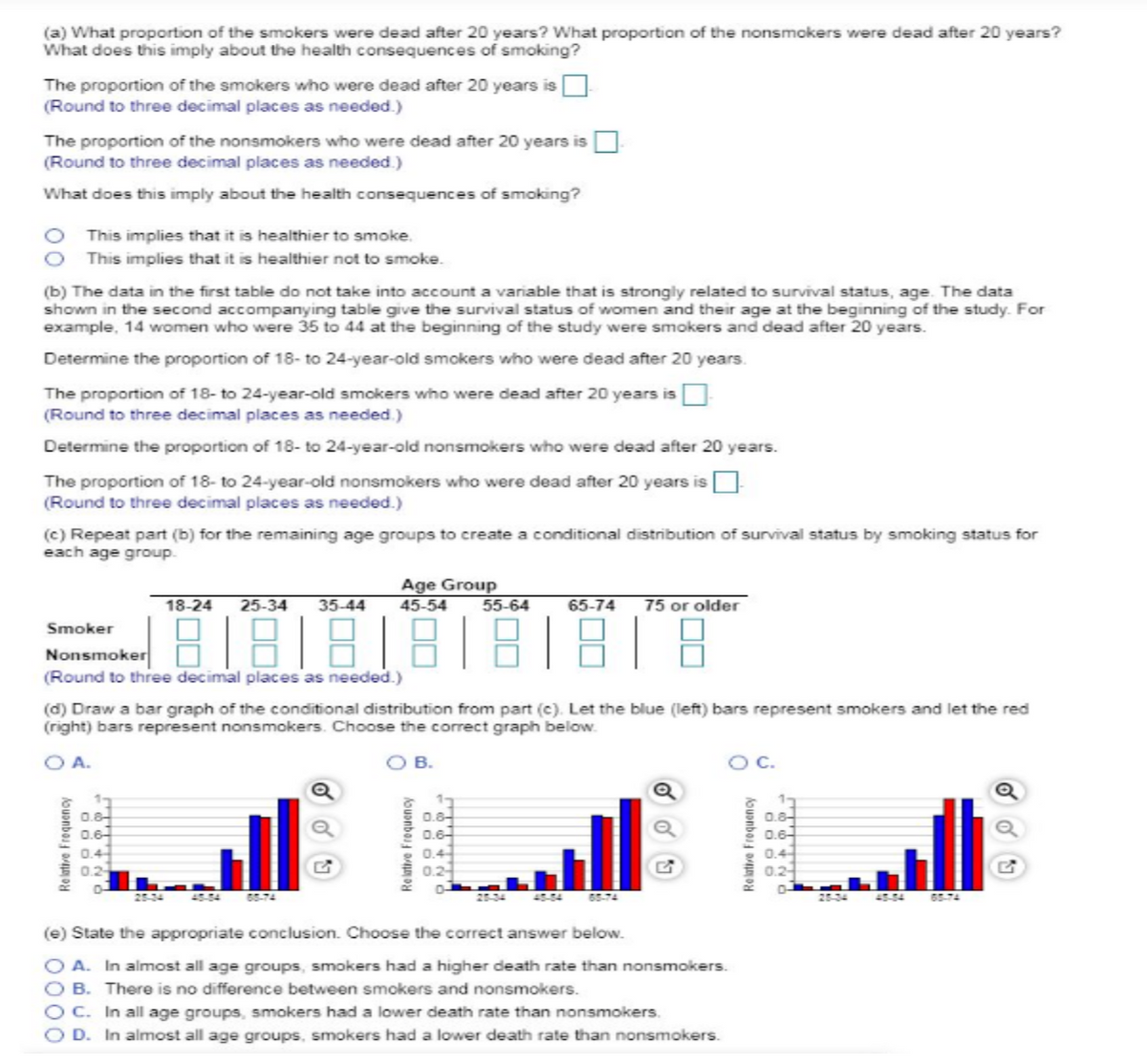
Could it be that smoking actually increases survival rates among women? The accompanying data represent the 20-year survival status and smoking status of
1334 women who participated in a 20-year cohort study. Complete parts (a) through (e).

Transcribed Image Text:O A.
(a) What proportion of the smokers were dead after 20 years? What proportion of the nonsmokers were dead after 20 years?
What does this imply about the health consequences of smoking?
The proportion of the smokers who were dead after 20 years is
(Round to three decimal places as needed.)
The proportion of the nonsmokers who were dead after 20 years is
(Round to three decimal places as needed.)
What does this imply about the health consequences of smoking?
O This implies that it is healthier to smoke.
This implies that it is healthier not to smoke.
(b) The data in the first table do not take into account a variable that is strongly related to survival status, age. The data
shown in the second accompanying table give the survival status of women and their age at the beginning of the study. For
example, 14 women who were 35 to 44 at the beginning of the study were smokers and dead after 20 years.
Determine the proportion of 18- to 24-year-old smokers who were dead after 20 years.
The proportion of 18- to 24-year-old smokers who were dead after 20 years is
(Round to three decimal places as needed.)
Determine the proportion of 18- to 24-year-old nonsmokers who were dead after 20 years.
The proportion of 18- to 24-year-old nonsmokers who were dead after 20 years is
(Round to three decimal places as needed.)
(c) Repeat part (b) for the remaining age groups to create a conditional distribution of survival status by smoking status for
each age group.
18-24 25-34 35-44
Age Group
45-54
55-64
65-74 75 or older
Smoker
Nonsmoker
888888
(Round to three decimal places as needed.)
(d) Draw a bar graph of the conditional distribution from part (c). Let the blue (left) bars represent smokers and let the red
(right) bars represent nonsmokers. Choose the correct graph below.
Relative Frequency
0.8
0.6
0.4
0.2
O B.
Relative Frequency
0.8-
0.6-
0.4-
0.2
G
(e) State the appropriate conclusion. Choose the correct answer below.
OA. In almost all age groups, smokers had a higher death rate than nonsmokers.
OB. There is no difference between smokers and nonsmokers.
OC. In all age groups, smokers had a lower death rate than nonsmokers.
D. In almost all age groups, smokers had a lower death rate than nonsmokers.
OC.
Relative Frequency
0.8
0.6
0.4
0.2
-го
28-34
65-

Transcribed Image Text:Smoking Status
Smoker (S)
Nonsmoker (NS)
Dead
144
233
Alive
452
513
Age Group
18-24
25-34
35-44
45-54
55-64
65-74
75 or
older
S NS S
NS
S
NS
S
NS
S NS
S
NS
S NS
Dead 3 2 4 6
14
7
28 12
51
40 29 102
15 64
Alive 54 63 124 157
97
118
103 66
60
66
81
8
28
0
0
Expert Solution
This question has been solved!
Explore an expertly crafted, step-by-step solution for a thorough understanding of key concepts.

Step by stepSolved in 3 steps with 1 images

Knowledge Booster

Similar questions
- Question C). Please make sure your answer is correct, I have been wrong twice. Thankssssss!!!!arrow_forward2. Metal Tags on Penguins and Survival. Data were collected over a 10-year timespan from a sample of 100 penguins that were randomly given either metal or electronic tags. One variable examined is the survival rate 10 years after tagging. The scientists observed that 10 of the 50 metal tagged penguins survived, compared to 18 of the 50 electronic tagged penguins. Test whether the survival rate is lower among metal- tagged penguins than among electronic-tagged penguins. Use subscripts E for Electronic and M for Metal. a. State hypotheses. b. Calculate the sample statistic PE - PM c. Use Normal distribution methods to calculate a z-test statistic, given SE = 0.0898. d. Find the p-value and draw a Normal curve with z-statistic and appropriate shaded region. Normal curve: p-value: e. State the conclusion of the test in context, using nontechnical language. f. Find a 90% confidence interval to three decimal places for this difference in proportions, given SE= 0.08836. Show your…arrow_forwardIn a survey of working parents (both parents working), one of the questions asked was "Have you refused a job, promotion, or transfer because it would mean less time with your family?" Two hundred men and 200 women were asked this question. Twenty-nine percent of the men and 24% of the women responded "yes." a. Based on this survey, can we conclude that there is a difference in the proportion of man and women responding “yes" at the 0.05 level of significance? (i) State the null and alternative hypotheses (ii) What test statistics would you use and why? (iii) Compute the value of the test-statistic. (iv) What rejection region would you use? (v) State your conclusion in the context of the problem. b. What P-value is associated with this test? Based on this P-value, could H. be rejected at significance level 0.08? c. Find a 95% confidence interval for the difference between the proportion of men and women responding "yes." Based on this confidence interval, would your conclusion be the…arrow_forward
- Education influences attitude and lifestyle. Differences in education are a big factor in the "generation gap." Is the younger generation really better educated? Large surveys of people age 65 and older were taken in n1 = 38 U.S. cities. The sample mean for these cities showed that x1 = 15.2% of the older adults had attended college. Large surveys of young adults (age 25 - 34) were taken in n2 = 37 U.S. cities. The sample mean for these cities showed that x2 = 18.1% of the young adults had attended college. From previous studies, it is known that ?1 = 6.4% and ?2 = 4.8%. Does this information indicate that the population mean percentage of young adults who attended college is higher? Use ? = 0.05. What is the value of the sample test statistic? (Test the difference ?1 − ?2. Round your answer to two decimal places.)=__(c) Find (or estimate) the P-value. (Round your answer to four decimal places.)=__arrow_forwardIn a study of how depression may affect one's ability to survive a heart attack, the researchers reported the ages of the two groups they examined. The mean age of 2397 patients without cardiac disease was 69.8 years, while for the 450 patients with cardiac disease, the mean age was 74.0, respectively. Furthermore, 32% of the diseased group were smokers, compared with only 23.7% of those free of heart disease. (1) Determine a 96% confidence interval for the difference in the proportions of smokers in the two groups. (ii) Indicate whether the two groups in the study were different. State the assumptions in order to proceed with the confident interval construction. (ii)arrow_forwardThe price of a share of stock divided by the company's estimated future earnings per share is called the P/E ratio. High P/E ratios usually indicate "growth" stocks, or maybe stocks that are simply overpriced. Low P/E ratios indicate "value" stocks or bargain stocks. A random sample of 51 of the largest companies in the United States gave the following P/E ratiost. 9 20 11 35 19 13 15 21 29 53 16 26 21 14 21 27 10 12 47 14 40 18 60 72 33 14 8 49 5 16 8 19 12 31 67 51 26 18 17 20 19 13 25 23 27 44 20 27 19 18 32 (a) Use a calculator with mean and sample standard deviation keys to find the sample mean x and sample standard deviation s. (Round your answers to one decimal place.) (b) Find a 90% confidence interval for the P/E population mean u of all large U.S. companies. (Round your answers to one decimal place.) lower limit upper limit (c) Find a 99% confidence interval for the P/E population mean u of all large U.S. companies. (Round your answers to one decimal place.) lower limit upper…arrow_forward
- Education influences attitude and lifestyle. Differences in education are a big factor in the "generation gap." Is the younger generation really better educated? Large surveys of people age 65 and older were taken in n1 = 38 U.S. cities. The sample mean for these cities showed that x1 = 15.2% of the older adults had attended college. Large surveys of young adults (age 25 - 34) were taken in n2 = 37 U.S. cities. The sample mean for these cities showed that x2 = 18.1% of the young adults had attended college. From previous studies, it is known that ?1 = 6.4% and ?2 = 4.8%. Does this information indicate that the population mean percentage of young adults who attended college is higher? Use ? = 0.05. (c) Find (or estimate) the P-value. (Round your answer to four decimal places.) A random sample of n1 = 12 winter days in Denver gave a sample mean pollution index x1 = 43. Previous studies show that ?1 = 15. For Englewood (a suburb of Denver), a random sample of n2 = 16 winter days gave a…arrow_forwardTourism is extremely important to the economy of Florida. Hotel occupancy is an often-reported measure of visitor volume and visitor activity (Orlando Sentinel, May 19, 2018). Hotel occupancy data for February in two consecutive years are as follows. Current Year Previous Year Occupied Rooms 1,360 1,386 Total Rooms 1,700 1,800 a. Formulate the hypothesis test that can be used to determine whether there has been an increase in the proportion of rooms occupied over the one-year period. Let pi = population proportion of rooms occupied for current year Pa= population proportion of rooms occupied for previous year Ho : Pi - Pa H.: Pi - P2 Select your answer Select your answer b. What is the estimated proportion of hotel rooms occupied each year (to 2 decimals)? Current year Previous Year c. Conduct a hypothesis test. What is the p-value (to 4 decimals)? Use Table 1 from Appendix B. p-value - Using a 0.05 level of significance, what is your conclusion? We Select your answer- vthat there has…arrow_forwardCheck My Work (5 remaining) Each year, over 2 million people in the United States become infected with bacteria that are resistant to antibiotics. In particular, the Centers of Disease Control and Prevention has launched studies of drug-resistant gonorrhea (CDC.gov website). Of 142 cases tested in Alabama, 9 were found to be drug-resistant. Of 268 cases tested in Texas, 5 were found to be drug-resistant. Do these data suggest a statistically significant difference between the proportions of drug- resistant cases in the two states? Use a 0.02 level of significance. What is the p-value, and what is your conclusion? Test statistic = (to 2 decimals) p-value = (to 4 decimals) Conclusion: Reject the null hypothesis Choose the correct option. There is a significant difference in drug resistance between the two states. Alabama has the higher drug resistance rate. Truearrow_forward
arrow_back_ios
arrow_forward_ios
Recommended textbooks for you
- MATLAB: An Introduction with ApplicationsStatisticsISBN:9781119256830Author:Amos GilatPublisher:John Wiley & Sons Inc
 Probability and Statistics for Engineering and th...StatisticsISBN:9781305251809Author:Jay L. DevorePublisher:Cengage Learning
 Statistics for The Behavioral Sciences (MindTap C...StatisticsISBN:9781305504912Author:Frederick J Gravetter, Larry B. WallnauPublisher:Cengage Learning
  Elementary Statistics: Picturing the World (7th E...StatisticsISBN:9780134683416Author:Ron Larson, Betsy FarberPublisher:PEARSON
 The Basic Practice of StatisticsStatisticsISBN:9781319042578Author:David S. Moore, William I. Notz, Michael A. FlignerPublisher:W. H. Freeman
 Introduction to the Practice of StatisticsStatisticsISBN:9781319013387Author:David S. Moore, George P. McCabe, Bruce A. CraigPublisher:W. H. Freeman
MATLAB: An Introduction with Applications
Statistics
ISBN:9781119256830
Author:Amos Gilat
Publisher:John Wiley & Sons Inc
Probability and Statistics for Engineering and th...
Statistics
ISBN:9781305251809
Author:Jay L. Devore
Publisher:Cengage Learning
Statistics for The Behavioral Sciences (MindTap C...
Statistics
ISBN:9781305504912
Author:Frederick J Gravetter, Larry B. Wallnau
Publisher:Cengage Learning
Elementary Statistics: Picturing the World (7th E...
Statistics
ISBN:9780134683416
Author:Ron Larson, Betsy Farber
Publisher:PEARSON
The Basic Practice of Statistics
Statistics
ISBN:9781319042578
Author:David S. Moore, William I. Notz, Michael A. Fligner
Publisher:W. H. Freeman
Introduction to the Practice of Statistics
Statistics
ISBN:9781319013387
Author:David S. Moore, George P. McCabe, Bruce A. Craig
Publisher:W. H. Freeman