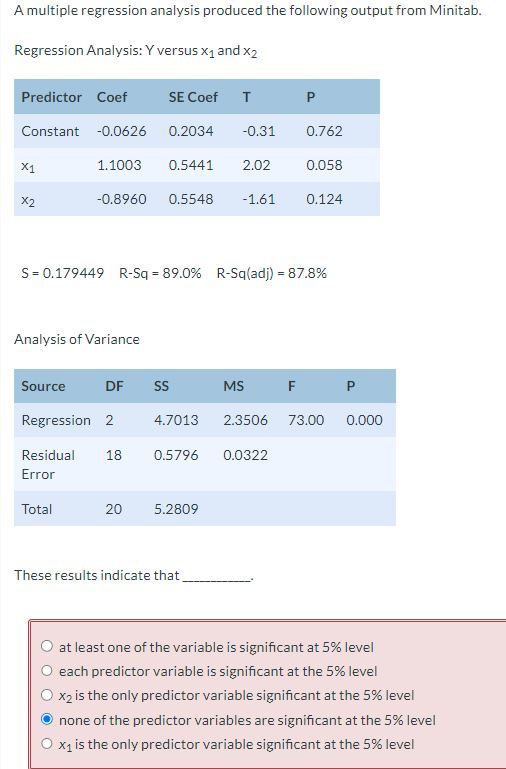
A multiple regression analysis produced the following output from Minitab. Regression Analysis: Y versus X₁ and x2 Predictor Coef Constant -0.0626 0.2034 X1 X2 Analysis of Variance SE Coef T 1.1003 0.5441 2.02 -0.8960 0.5548 -1.61 Source DF Regression 2 Residual 18 Error Total 20 S=0.179449 R-Sq - 89.0 % R-Sq(adj) = 87.8% SS -0.31 0.5796 0.0322 5.2809 P MS F P 4.7013 2.3506 73.00 0.000 These results indicate that. 0.762 0.058 0.124 at least one of the variable is significant at 5% level each predictor variable is significant at the 5% level X₂ is the only predictor variable significant at the 5% level none of the predictor variables are significant at the 5% level O x₁ is the only predictor variable significant at the 5% level

You are interested in how the number of hours a high school student has to work in an outside job has on their GPA. In your regression you want to control for high school standing and so you run the following regression: GPA = 3.4 0.03 * HrsWrk - 0.7 * Frosh - 0.3 * Soph +0.1 * Junior (1.1) (0.013) (0.23) (0.14) (0.08) where HrsWrk is the number of hours the student works per week, and Frosh, Soph, and Junior are dummy variables for the student's class standing. a) If you include a dummy variable for seniors, that would cause a Hint: type one word in each blank. For the rest of questions, type a number in one decimal place. b) The expected GPA of a Sophomore who works 10 hours per week is c) The expected GPA of a Senior who works 10 hours per week is d) If Dom and Sarah work the same number of hours per week, but Dom is a Junior and Sarah is a Freshman. Dom is expected to have a higher GPA than Sarah. e) Suppose you rewrite the regression as: problem. GPA = ₁HrsWrk + ß2Frosh + B2Soph +…

Help!

Please provide the correct answer along with the calculation. Do not use ChatGPT, otherwise I will give a downvote.