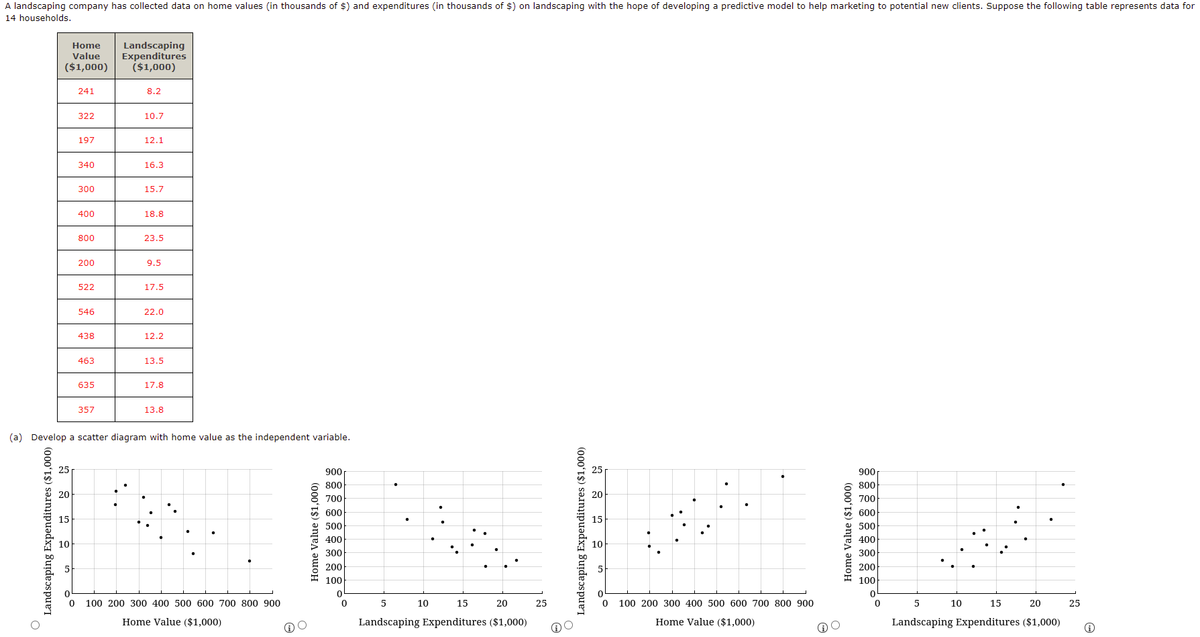
A landscaping company has collected data on home values (in thousands of $) and expenditures (in thousands of $) on landscaping with the hope of developing a predictive model to help marketing to potential new clients. Suppose the following table represents data for 14 households. Landscaping Expenditures ($1,000) Home Value ($1,000) 241 8.2 322 10.7 197 12.1 340 16.3 300 15.7 400 18.8 80 23.5 200 9.5 522 17.5 546 22.0 438 12.2 463 13.5 635 17.8 357 13.8 (a) Develop a scatter diagram with home value as the independent variable. - 25 900 900 800 700 * 600 500 800 320 20 700 600 15 15 500 400 400 蓋 101 10 300 200 * 100 300 200 100 O 100 200 300 400 500 600 700 800 900 10 15 20 25 100 200 300 400 500 600 700 800 900 10 15 20 25 Home Value ($1,000) Landscaping Expenditures ($1,000) Home Value ($1,000) Landscaping Expenditures ($1,000) Landscaping Expenditures ($1,000) Home Value ($1,000) Landscaping Expenditures ($1,000) Home Value ($1,000)

Suppose you are conducting a study about how the average US worker spends time over the course of a workday. You are interested in how much time workers spend per day on personal calls, emails, and social networking websites, as well as how much time they spend socializing with coworkers versus actually working. The most recent census provides data for the entire population of US workers on variables such as travel time to work, time spent at work, and break time at work. The census, however, does not include data on the variables you are interested in, so you obtain a random sample of 102 full-time workers in the United States and ask about personal calls, emails, and so forth. You are curious about how your sample compares with the census, so you also ask the workers the same questions about work that are asked in the census. Suppose the mean travel time to work from the most recent census is 24.1 minutes, with a standard deviation of 4.5 minutes. Your sample of 102 US workers…

The data below lists states poverty rate, gun deaths per 100,000 people, high school graduation rate and the unemployment rate. STATE New Jersey Vermont Minnesota Hawaii Delaware Utah Virginia Nebraska Connecticut Maryland Idaho Alaska Massachusetts Washington Wisconsin Nevada Wyoming Florida North Dakota Pennsylvania lowa Colorado Illinois Missouri South Dakota Michigan New Hampshire Rhode Island Ohio Kansas POVERTY% 6.80% 7.60% 8.10% 8.60% 9.20% 9.20% 9.20% 9.50% 9.70% 9.70% 9.90% 10.00% 10.10% 10.20% 10.20% 10.60% 10.60% 11.10% 11.20% 11.20% 11.30% 11.40% 11.50% 11.60% 11.80% 12.00% 12.00% 12.10% 12.30% 12.50% GUN DEATHS 5.7 9.2 12 2.6 10.3 12.6 10.2 9 4.4 9.7 14.1 17.6 3.1 8.7 9.7 13.8 16.7 11.9 11.8 11.2 8 11.5 8.6 12 10 12 6.4 5.3 11 11.4 H.S. GRAD's 91.8 91 91.5 90.4 87.4 90.4 86.6 89.8 88.6 88.2 88.4 91.4 89 89.7 89.8 83.9 87.4 85.3 90.1 87.9 91.4 89.3 86.4 86.8 89.9 87.9 91.3 84.7 87.6 89.7 UNEMPLOYMENT 5.7 3.6 4 3.5 4.9 3.7 4.5 2.8 5.3 5.1 4.2 6.6 4.7 5.3 4.5 6.8 4 5.3 2.9…

TYPEWRITTEN ONLY PLEASE FOR UPVOTE. DOWNVOTE FOR HANDWRITTEN. DO NOT ANSWER IF YOU ALREADY ANSWERED THIS. I'LL DOWNVOTE.

A psychologist believed that as children get older, they engage in more “inactive activities” such as playing computer games, watching TV and surfing the internet. She collected data from 10 children. She recorded the age of each child and the amount of activity (in hours) the child engaged in per week.  Age Activity 7 4.3 9 3.2 10 1 13 1.5 12 1.2 15 0.8 9 3 12 4 15 1.5 14 1.9   Using excel, obtain a scatterplot of the data. Discuss the relationship between age and activity based on the scatterplot. Using excel, obtain the simple linear regression linear regression line predicting activity from age. Interpret the intercept and slope of the regression line. By hand, predict the amount of activity for age = 14. By hand, calculate the residual for age = 14 Using excel output, test the null hypothesis that the slope coefficient is zero using the p-value approach. Write one sentence interpreting the meaning of this result. Make sure to report the test statistic…