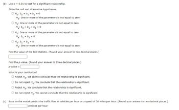
(b) Use a = 0.01 to test for a significant relationship.State the null and alternative hypotheses.Ho: bo = b₁ = b ₂ = 0H₂: One or more of the parameters is not equal to zero.O Ho: One or more of the parameters is not equal to zero.Ha: bo=b₁ = b ₂ = 0O Ho: One or more of the parameters is not equal to zero.Ha: b₁ b₂ = 0ⒸH₁: b₁ = b ₂ = 0H₂: One or more of the parameters is not equal to zero.Find the value of the test statistic. (Round your answer to two decimal places.)Find the p-value. (Round your answer to three decimal places.)p-value =What is your conclusion?O Reject Ho. We cannot conclude that the relationship is significant.Do not reject Ho. We conclude that the relationship is significant.O Reject Ho. We conclude that the relationship is significant.O Do not reject Ho. We cannot conclude that the relationship is significant.(c) Base on the model predict the traffic flow in vehicles per hour at a speed of 38 miles per hour. 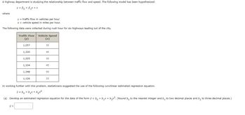(Round your answer to two decimal places.)vehicles per hour A highway department is studying the relationship between traffic flow and speed. The following model has been hypothesized:y =B₁ + B₁x + 8wherey = traffic flow in vehicles per hourx = vehicle speed in miles per hour.The following data were collected during rush hour for six highways leading out of the city.Traffic Flow Vehicle Speed(y)(x)1,257351,330401,225301,334451,348501,12625In working further with this problem, statisticians suggested the use of the following curvilinear estimated regression equation.ŷ = bo + b₂x + b₂x²(a) Develop an estimated regression equation for the data of the form ý = bo + b₁x + b₂x². (Round bo to the nearest integer and b₁ to two decimal places and b₂ to three decimal places.)

Answered: Image /qna-images/answer/76e8f277-b013-4f81-bb3c-8eef187b4e66.jpg

A highway department is studying the relationship between traffic flow and speed. The following model has been hypothesized: y =B₁ + B₁x + 8 where y = traffic flow in vehicles per hour x = vehicle speed in miles per hour. The following data were collected during rush hour for six highways leading out of the city. Traffic Flow Vehicle Speed (y) (x) 1,257 35 1,330 40 1,225 30 1,334 45 1,348 50 1,126 25 In working further with this problem, statisticians suggested the use of the following curvilinear estimated regression equation. ŷ = bo + b₁x + b₂x² (a) Develop an estimated regression equation for the data of the form ý = bo + b₂x + b₂x². (Round bo to the nearest integer and b₁ to two decimal places and b₂ to three decimal places.) ý =

A highway department is studying the relationship between traffic flow and speed. The following model has been hypothesized: y =B₁ + B₁x + 8 where y = traffic flow in vehicles per hour x = vehicle speed in miles per hour. The following data were collected during rush hour for six highways leading out of the city. Traffic Flow Vehicle Speed (y) (x) 1,257 35 1,330 40 1,225 30 1,334 45 1,348 50 1,126 25 In working further with this problem, statisticians suggested the use of the following curvilinear estimated regression equation. ŷ = bo + b₁x + b₂x² (a) Develop an estimated regression equation for the data of the form ý = bo + b₂x + b₂x². (Round bo to the nearest integer and b₁ to two decimal places and b₂ to three decimal places.) ý =

College Algebra

7th Edition

ISBN:9781305115545

Author:James Stewart, Lothar Redlin, Saleem Watson

Publisher:James Stewart, Lothar Redlin, Saleem Watson

Chapter1: Equations And Graphs

Section: Chapter Questions

Problem 10T: Olympic Pole Vault The graph in Figure 7 indicates that in recent years the winning Olympic men’s...

See similar textbooks

Similar questions

Olympic Pole Vault The graph in Figure 7 indicates that in recent years the winning Olympic men’s pole vault height has fallen below the value predicted by the regression line in Example 2. This might have occurred because when the pole vault was a new event there was much room for improvement in vaulters’ performances, whereas now even the best training can produce only incremental advances. Let’s see whether concentrating on more recent results gives a better predictor of future records. (a) Use the data in Table 2 (page 176) to complete the table of winning pole vault heights shown in the margin. (Note that we are using x=0 to correspond to the year 1972, where this restricted data set begins.) (b) Find the regression line for the data in part ‚(a). (c) Plot the data and the regression line on the same axes. Does the regression line seem to provide a good model for the data? (d) What does the regression line predict as the winning pole vault height for the 2012 Olympics? Compare this predicted value to the actual 2012 winning height of 5.97 m, as described on page 177. Has this new regression line provided a better prediction than the line in Example 2?
The following estimated regression model was developed relating yearly income (y in $1000s) of 30 individuals with their age (x1) and their gender (x2) (0 if male and 1 if female).ŷ = 30 + 0.7x1 + 3x2Also provided are SST = 1200 and SSE = 384.The yearly income of a 24-year-old female individual is _____.
The table presents data on the taste test of 38 brands of pinot noir wine [data were first reported in an article by Kwan, Kowalski, and Skogenboe in the Journal Agricultural and Food Chemistry (1979, Vol. 27), the response variable is y = quality, and we want to find the "best" regression equation that relates quality to the other five parameters
The table contains data on vehicle speed (h) and fuel consumption (lt / 100km) of 5 randomly selected vehicles. Estimate the average fuel consumption of a vehicle traveling at 45 km / h using the simple linear regression equation between vehicle speed and fuel consumption. Speed 55 60 65 70 75 Consumption 11 10 9 8 7 Please choose one: a. 6 b. 5 c. 13 D. 8
The table contains data on vehicle speed (h) and fuel consumption (lt / 100km) of 5 randomly selected vehicles. Estimate the average fuel consumption of a vehicle traveling at 45 km / h using the simple linear regression equation between vehicle speed and fuel consumption. Speed 55 60 65 70 75 Consumption 13 12 11 10 9 a. 15 b. 8 c. 7 d. 20
The birth lengths in cm (x) and birth weights in kg (y) of a sample of 50 newborn female babies are compared, yielding a correlation coefficient of r=0.578 and a linear regression equation of ŷ =−8.89+0.243x The babies all had lengths between 46.5 and 53.0 cm, and weights between 2.50 and 4.05 kg. Based on this, predict the birth weight of a newborn female baby with a birth length of 48.5 cm.
The table below shows the number of state-registered automatic weapons and the murder rate for several Northwestern states. xx 11.7 8.4 7 3.8 2.7 2.3 2.5 0.3 yy 14.2 11.4 10.2 7.4 6.3 6.1 6 4 xx = thousands of automatic weaponsyy = murders per 100,000 residentsThis data can be modeled by the equation ˆy=0.89x+3.89.y^=0.89x+3.89. Use this equation to answer the following;Note: Verify this equation using your calculator.A) How many murders per 100,000 residents can be expected in a state with 2.8 thousand automatic weapons?Answer = Round to 3 decimal places.B) How many murders per 100,000 residents can be expected in a state with 8.5 thousand automatic weapons?Answer = Round to 3 decimal places.
It is known that the linear regression equation: y= -2.88+1.77x, with a coefficient of determination of 0.81. Based on the two information, the correlation coefficient is
For the regression model Yi = b0 + eI, derive the least squares estimator.
The owner of Original Italian Pizza restaurant chain wants to understand which variable most strongly influences the sales of his specialty deep-dish pizza. He has gathered data on the monthly sales of deep-dish pizzas at his restaurants and observations on other potentially relevant variables for each of several outlets in central Indiana. These data are provided in the file P10_04.xlsx. Estimate a simple linear regression equation between the quantity sold (Y) and each of the following candidates for the best explanatory variable: average price of deep-dish pizzas (X1), monthly advertising expenditures (X2), and disposable income per household in the areas surrounding the outlets (X3). Round your answers for intercept coefficients to the nearest whole number and slope coefficients to two decimal places, if necessary. If your answer is negative number, enter "minus" sign.
Suppose that researchers are interested in determining the bi-annual salary of statisticians of different levels using their years of experience and their education level (M = bachelors, P = doctorate). They fit the following model to a dataset that includes these variables and, after performing the proper steps of multiple linear regression, the following multiple linear regression model is obtained: yˆ = 42308 + 323x1 + 213x2 + 301(x1*x2) where the variables are as follows: yˆ = predicted bi−annual salary in dollars, x1 = number of years of experiencex2= {1 if the education level is a doctorate 0 if the education level is a bachelors What is the predicted bi-annual salary in dollars of an employee with 5 years of experience and a bachelor’s degree?
Suppose that researchers are interested in determining the bi-annual salary of statisticians of different levels using their years of experience and their education level (M = bachelors, P = doctorate). They fit the following model to a dataset that includes these variables and, after performing the proper steps of multiple linear regression, the following multiple linear regression model is obtained: yˆ = 42308 + 323x1 + 213x2 + 301(x1*x2) where the variables are as follows: yˆ = predicted bi−annual salary in dollars, x1 = number of years of experiencex2= {1 if the education level is a doctorate 0 if the education level is a bachelors What is the predicted bi-annual starting salary of an employee with a doctorate degree? (Someone with no work experience). $ What is the predicted bi-annual starting salary of an employee with a bachelor’s degree? (Someone with no work experience). $