MATLAB: An Introduction with Applications
6th Edition
ISBN: 9781119256830
Author: Amos Gilat
Publisher: John Wiley & Sons Inc
expand_more
expand_more
format_list_bulleted
Question

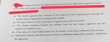
Transcribed Image Text:5.
Indicate if each of the following statements about the simple linear regression model is
true or false and explain why.
(a). The simple regression line estimated by the method of Least Squared passes through the
sample mean of dependent and independent variable.
(b). The slope estimator of the Least Squares regression line is free of measure.
(c). The sample covariance between the residuals from the least square regression and the
explanatory variable is zero.
(d). If the values of x more widely spread out, the estimate of the slope coefficient is less concise.
(e). Adjusted R-squared will always increase when an additional independent variable is added into
the regression.
Expert Solution
This question has been solved!
Explore an expertly crafted, step-by-step solution for a thorough understanding of key concepts.
Step by stepSolved in 3 steps

Knowledge Booster
Similar questions
- Q2. The Update to the Task Force Report on Blood Pressure Control in Children reported the observedaverage SBP in single years of age from age 1 to 17 based on prior studies. The data for boys of averageSBP at each age are given in HW 5 data.sav on Blackboard. Suppose we seek a more efficient way todisplay the data and choose linear regression to accomplish this task.1) Fit a regression line using age as independent variable and SBP as dependent variable. (Theappropriate output is required here if you used software)2) Interpret the regression equation.3) Provide and interpret a 90% confidence interval for the parameters of the regression line.4) Perform ANOVA test for the population slope. Use α = 0.05, and both rejection region and p-value to make a decision.5) What the predicted (estimated) blood pressure on average is for a 10-year-old boy as estimatedfrom the regression line?6) Interpret R2.7) Check the conditions for your regression analysis using the appropriate plots. Age…arrow_forward#3. What is the least squares regression line for the following set of data? y-hat = 2.18x + 27.74 y-hat = 2.14x + 27.44 y-hat = 1.94x + 26.24 y-hat =1.86x + 26.28arrow_forward(b)arrow_forward
- If a regression line for two variables has a small positive slope, then the: variables are positively associated? variables are negatively associated? association of the variables cannot be determined. variables have no association with each other.arrow_forward4. We would like to determine how a man's weight can be used to predict his systolic blood pressure. We measure the weights (in pounds) and the systolic blood pressures of a sample of 17 men. The data are plotted on a scatterplot and it can be seen that a linear relationship is a reasonable assumption. The least squares regression line is calculated to be ŷ = 125.561 + 0.145x. The ANOVA table (with some values missing) is shown below: |Source of Variation | df | Sum of Squares Mean Square F Regression Error Total 26.46 617.82 (a) We would like to test whether a linear relationship exists between a man's weight and his systolic blood pressure. We will conduct an analysis of variance to test Ho: B1 = 0 vs. Ha: B1 + 0 at the 5% level of significance. Enter all missing values in the ANOVA table. Calculate the value of the test statistic, find the P-value of the test and provide a properly worded conclusion. (b) What is the value of the correlation between weight and systolic blood pressure…arrow_forward1arrow_forward
- You forgot to JUSTIFY THE ANSWRRS LAST TIMEarrow_forwardThe accompanying scatterplot shows the relationship between the age of an internet user and the amount of time spent browsing the internet per week (in minutes). The accompanying residual plot is also shown along with the QQ plot of the residuals. Choose the statement that best describes whether the condition for Normality of errors does or does not hold for the linear regression model. Choose the statement that best describes whether the condition for Normality of errors does or does not hold for the linear regression model. A.The residual plot displays a fan shape; therefore the Normality condition is not satisfied.B.The QQ plot mostly follows a straight line; therefore the Normality condition is satisfied.C.The scatterplot shows a negative trend; therefore the Normality condition is satisfied.D.The residual plot shows no trend; therefore the Normality condition is not satisfied.arrow_forward
arrow_back_ios
arrow_forward_ios
Recommended textbooks for you
 MATLAB: An Introduction with ApplicationsStatisticsISBN:9781119256830Author:Amos GilatPublisher:John Wiley & Sons Inc
 Probability and Statistics for Engineering and th...StatisticsISBN:9781305251809Author:Jay L. DevorePublisher:Cengage Learning
 Statistics for The Behavioral Sciences (MindTap C...StatisticsISBN:9781305504912Author:Frederick J Gravetter, Larry B. WallnauPublisher:Cengage Learning
 Elementary Statistics: Picturing the World (7th E...StatisticsISBN:9780134683416Author:Ron Larson, Betsy FarberPublisher:PEARSON
 The Basic Practice of StatisticsStatisticsISBN:9781319042578Author:David S. Moore, William I. Notz, Michael A. FlignerPublisher:W. H. Freeman
 Introduction to the Practice of StatisticsStatisticsISBN:9781319013387Author:David S. Moore, George P. McCabe, Bruce A. CraigPublisher:W. H. Freeman

MATLAB: An Introduction with Applications
Statistics
ISBN:9781119256830
Author:Amos Gilat
Publisher:John Wiley & Sons Inc

Probability and Statistics for Engineering and th...
Statistics
ISBN:9781305251809
Author:Jay L. Devore
Publisher:Cengage Learning

Statistics for The Behavioral Sciences (MindTap C...
Statistics
ISBN:9781305504912
Author:Frederick J Gravetter, Larry B. Wallnau
Publisher:Cengage Learning

Elementary Statistics: Picturing the World (7th E...
Statistics
ISBN:9780134683416
Author:Ron Larson, Betsy Farber
Publisher:PEARSON

The Basic Practice of Statistics
Statistics
ISBN:9781319042578
Author:David S. Moore, William I. Notz, Michael A. Fligner
Publisher:W. H. Freeman

Introduction to the Practice of Statistics
Statistics
ISBN:9781319013387
Author:David S. Moore, George P. McCabe, Bruce A. Craig
Publisher:W. H. Freeman