
Elements Of Electromagnetics
7th Edition
ISBN: 9780190698614
Author: Sadiku, Matthew N. O.
Publisher: Oxford University Press
expand_more
expand_more
format_list_bulleted
Related questions
Question
Can you help me code the algorithm into MATLAB? The delta zero, delta one and so forth are equal to the determinats of a 3x3 matrix made of the three
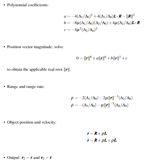

Transcribed Image Text:Polynomial coefficients:
• Position vector magnitude: solve
a =
4(A1/Ao)²+4(A1/Ao)L-R - ||R||²
b=-8µ(A/Ao)(A2/Ao)+4µ(A2/Ao)L-R
c=-4μ²(A2/Ao)²
to obtain the applicable real root ||r||.
(=r³+ar6+b||r||³+c
• Range and range-rate:
p -2(A/Ao)-2u||||³ (A2/Ao)
p=-(A3/Ao) - µ||||³ (A4/A0)
•
Object position and velocity:
r=R+PL
r=R+PL+PL
Output: 2 and v₂ =ŕ

Transcribed Image Text:3.1.3.1 Algorithm for Laplace's Method
.
Given: ti, Li, and R; for i€ {1,2,3} and
⚫ Observer position at middle observation: R = R₂
.
Observer velocity and acceleration: R-XR and R= × R
Lagrange interpolation coefficients:
$1
12-13
(11-12) (11-13)'
212-11-13
$2=
" $3=
2
(12-11) (12-13)
2
12-11
(13-11)(13-12)
2
S4=
$5
(11-12) (11-13)
"
(12-11)(12-13)
$6
"
(13-11)(13-12)
•
Line-of-sight and associated rates:
⚫ Determinants:
L-L2
L=S₁L₁+82L2+$3L3
L=84L1+55L2+8643
Ao 2|| L| L| | ||
=
ALL R ||
A2 L L
R ||
=
A3|L|R| L ||
ALR £ ||
Expert Solution
This question has been solved!
Explore an expertly crafted, step-by-step solution for a thorough understanding of key concepts.

Step by stepSolved in 2 steps

Knowledge Booster

Similar questions
- I want to run the SGP4 propagator for the ISS (ID = 25544) I got from spacetrack.org in MATLAB. I don't know where to get the inputs of the function. Where do I get the inFile and outFile that is mentioned in the following function. % Purpose: % This program shows how a Matlab program can call the Astrodynamic Standard libraries to propagate % satellites to the requested time using SGP4 method. % % The program reads in user's input and output files. The program generates an % ephemeris of position and velocity for each satellite read in. In addition, the program % also generates other sets of orbital elements such as osculating Keplerian elements, % mean Keplerian elements, latitude/longitude/height/pos, and nodal period/apogee/perigee/pos. % Totally, the program prints results to five different output files. % % % Usage: Sgp4Prop(inFile, outFile) % inFile : File contains TLEs and 6P-Card (which controls start, stop times and step size) % outFile : Base name for five output files %…arrow_forwardDon't Use Chat GPT Will Upvote And Give Handwritten Solution Pleasearrow_forwardZVA @ e SIM a A moodle1.du.edu.om Solve the second order homogeneous differential equation y " -6y'-7y = 0 with intial values y(0) = 0; y'(0) = 1 %3D Maximum file size: 200MB, maximum number of files: 1 Files IIarrow_forward
- H.W: suppose that a team of three parachutists are connected by a weightless cord while free falling at a velocity of 5 m/s. Using Gauss Elimination Method calculate the tension in each section of cord and the acceleration of the team, given the following information: 3 Parachutist Mass Kg(m) Drag Coefficient Kg/s (c) a 1 70 10 2 60 14 3 40 17 1 Hint: The equation of motion can be determine from Newton's Second Law (Σ F = ma). m₁g-Tc₁v = m₁a m₂g + T-R-C₂v = m₂a m3g+ R-C3v = mza R T 2arrow_forward= MMB 241- Tutorial 1.pdf 2/3 80% + + 10. Determine a ats = 1 m v (m/s) 4 s (m) 2 11. Draw the v-t and s-t graphs if v = 0, s=0 when t=0. a (m/s²) 2 t(s) 12. Draw the v-t graph if v = 0 when t=0. Find the equation v = f(t) for each a (m/s²) 2 segment. 2 -2 13. Determine s and a when t = 3 s if s=0 when t = 0. v (m/s) 2 t(s) t(s) 2arrow_forward'p' (liquid density 'A' (tank cross sectional area) 'Qin' (Input Flow Rate) "Que P 'R' (restriction coefficient) '' (head of liquid) dh Qin = A + dt Figure 1 The single tank system (Figure 1) has been modelled by the first order differential equation given as equation. The equation describes the relationship between the input flow rate entering the tank and the head of liquid in the tank. ph R 5 m equation The following constants are provided: R = 40 Kpa s m², 4 = 10 m², p= 1001 kg m², and g = 9.81 m s A pump is suddenly switched on and provides a step input flow rate of 0.5 m³s¹. (1) Using Laplace Transforms, solve equation and provide an expression to show how the level in the tank will vary in time after the step input has been applied.arrow_forward
- Problem 1 (15 points) (Core Course Outcome 5)/MatlabGrader Write a function mySecond Derivative Order 3 that calculates the second derivative d²y/dx² of a data set (x, y) with at least third order accuracy at each data point. The data is equidistant in x with spacing h. The function input shall be ⚫y: one-dimensional column vector of y values ⚫h: scalar value of spacing h The function output shall be • d2y: column vector of the same size as y containing d²y/dx² Calculate d²y/dx² using only the following formulas that use the nomenclature of Table 8-1 and the lecture notes, but are different from the formulas listed there: f" (xi) 164f(xi) — 465f(xi+1) + 460ƒ (xi+2) − 170ƒ (xi+3) + 11f (xi+5) + O(h³) = 60h2 56f(xi−1) − 105f(xi) +40f(xi+1) + 10f(xi+2) − f(x+4) + O(h³) 60h² −5f(xi−2) +80f(xi−1) − 150f(xi) + 80f(xi+1) − 5ƒ(xi+2) (1) f"(xi) = (2) f"(xi) = +0(h) (3) 60h2 f"(xi) -2f(x-4)+5f(xi-3)+50f(xi-1) — 110f(xi) +57f(xi+1) = +0(h³) (4) 60h² f"(xi) = 57f(x-5) 230f(xi-4) + 290 f (xi-3)-235…arrow_forwardWrite a MatLab code to solve these 4 equationsarrow_forwardSimulink Assignment- Filling a Tank In fluid mechanics, the equation that models the fluid level in a tank is: dh 1 -(min Ap - mout) dt h is the water level of the tank A is the surface area of the bottom of the tank pis the density of the fluid Mim and mout are the mass flow rates of water in and out of the tank, the flow out is a function of the water level h: 1 mout Vpgh Ris the resistance at the exit. Assume that the exit is at the bottom of the tank. g is the gravitational acceleration What to Do: 1. Build a model in Simulink to calculate the water level, h, as a function of time. Your model should stop running as soon as the tank is full. 2. Assuming the height of the tank is 2 meters, after how many seconds does the tank fill up? Use the following constants to test your model: • A: area of the bottom of the tank = 1 m? • p: the density of fluid = 1000 kg/ m? • R: the resistance at the exit = 3 (kg.m)-1/2 • ho: Initial height of the fluid in the tank = 0 m • g: the gravitational…arrow_forward
arrow_back_ios
SEE MORE QUESTIONS
arrow_forward_ios
Recommended textbooks for you
- Elements Of ElectromagneticsMechanical EngineeringISBN:9780190698614Author:Sadiku, Matthew N. O.Publisher:Oxford University Press
 Mechanics of Materials (10th Edition)Mechanical EngineeringISBN:9780134319650Author:Russell C. HibbelerPublisher:PEARSON
 Thermodynamics: An Engineering ApproachMechanical EngineeringISBN:9781259822674Author:Yunus A. Cengel Dr., Michael A. BolesPublisher:McGraw-Hill Education
  Control Systems EngineeringMechanical EngineeringISBN:9781118170519Author:Norman S. NisePublisher:WILEY
 Mechanics of Materials (MindTap Course List)Mechanical EngineeringISBN:9781337093347Author:Barry J. Goodno, James M. GerePublisher:Cengage Learning
 Engineering Mechanics: StaticsMechanical EngineeringISBN:9781118807330Author:James L. Meriam, L. G. Kraige, J. N. BoltonPublisher:WILEY
Elements Of Electromagnetics
Mechanical Engineering
ISBN:9780190698614
Author:Sadiku, Matthew N. O.
Publisher:Oxford University Press
Mechanics of Materials (10th Edition)
Mechanical Engineering
ISBN:9780134319650
Author:Russell C. Hibbeler
Publisher:PEARSON
Thermodynamics: An Engineering Approach
Mechanical Engineering
ISBN:9781259822674
Author:Yunus A. Cengel Dr., Michael A. Boles
Publisher:McGraw-Hill Education
Control Systems Engineering
Mechanical Engineering
ISBN:9781118170519
Author:Norman S. Nise
Publisher:WILEY
Mechanics of Materials (MindTap Course List)
Mechanical Engineering
ISBN:9781337093347
Author:Barry J. Goodno, James M. Gere
Publisher:Cengage Learning
Engineering Mechanics: Statics
Mechanical Engineering
ISBN:9781118807330
Author:James L. Meriam, L. G. Kraige, J. N. Bolton
Publisher:WILEY