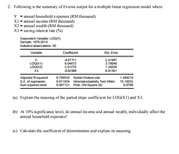
2. Following is the summary of Eviews output for a multiple linear regression model where Yannual household expenses (RM thousand) X1 = annual income (RM thousand) X2= annual wealth (RM thousand) X3 = saving interest rate (%) Dependent Variable: LOG(Y) Sample: 1970 2019 Included observations: 50 Variable с LOG(X1) LOG(X2) X3 Coefficient -4.67711 8.04873 2.01270 -0.02689 Adjusted R-squared S.E. of regression Sum squared resid Std. Error 2.41907 3.79049 1.24934 0.01361 0.789533 Durbin-Watson stat 0.011934 Heteroskedasticity Test White 0.007121 Prob. Chi-Square (6) (a) Explain the meaning of the partial slope coefficient for LOG(X1) and X3. 1.589219 10.16032 0.0708 (b) At 10% significance level, do annual income and annual wealth, individually affect the annual household expenses? (c) Calculate the coefficient of determination and explain its meaning.

Please briefly explain the results with explanation and clear points. Do not answer this of you want to copy and if you are not confident. Question - List the main results, and explain the intuition behind these results?

Suppose that a 5% rise in the price of apples does not cause the quantity demanded to change. The elasticityof demand for apples would then be: a. 0.b. –1.c. –2.d. infinitely large.

wages = B1 + B2educ + ßzexper + e where wages denotes hourly wages. We estimate the regression in R and obtain the output ## Coefficients: ## Estimate Std. Error t value Pr(>|t|) ## (Intercept) 2.0 1.0 2 0.0455 * ## educ 0.5 0.5 1 0.3173 ## exper 2.0 0.5 4 6.33e-05 *** ## --- ## Signif. codes: ****' 0. 001 '**' 0.01 **' 0.05 ' 0.1 ' ' 1 Build a 90% confidence interval for B3 using a normal approximation. (Use that if Z ~ N(0, 1) and z1-a satisfies P(Z > z1-a) = a, then zo9 = 1.28, zo95 = 1.64, Z0.975 = 1.96, zo.99 = 2.33, and z0.995 = 2.58). Oa. [2 – 1.64 x (0.5), 2 + 1.64 x (0.5)] O b. [2 – 1.28 × (0.5), 2 + 1.28 x (0.5)] c. [2 – 1.28 x (0.5)², 2 + 1.28 × (0.5)²] O d. [2 – 1.64 × (0.5)², 2 + 1.64 × (0.5)²] O e. [2 – 1.96 × (0.5)², 2 + 1.96 × (0.5)²] O f. [2 – 1.96 × (0.5), 2 + 1.96 × (0.5)]

q13-

You estimated a regression with the following output.         Source |       SS           df       MS      Number of obs   =       289 -------------+----------------------------------   F(1, 287)       =  41986.64        Model |   664544048         1   664544048   Prob > F        =    0.0000     Residual |  4542496.25       287  15827.5131   R-squared       =    0.9932 -------------+----------------------------------   Adj R-squared   =    0.9932        Total |   669086544       288  2323217.17   Root MSE        =    125.81   ------------------------------------------------------------------------------            Y |      Coef.   Std. Err.      t    P>|t|     [95% Conf. Interval] -------------+----------------------------------------------------------------            X |   43.81013   .2138056   204.91   0.000     43.38931    44.23096        _cons |   49.31707   16.96222     2.91   0.004     15.93094    82.70319…

In an OLS regression, which value represents the "best" R2 in terms of explained variance in the dependent variable?  A. 2.53 B. 16.22 C. .001 D. 0.53

Help!

You estimated a regression with the following output.         Source |       SS           df       MS      Number of obs   =       411 -------------+----------------------------------   F(1, 409)       =   4098.54        Model |  22574040.7         1  22574040.7   Prob > F        =    0.0000     Residual |  2252702.97       409  5507.83122   R-squared       =    0.9093 -------------+----------------------------------   Adj R-squared   =    0.9090        Total |  24826743.7       410  60553.0334   Root MSE        =    74.215   ------------------------------------------------------------------------------            Y |      Coef.   Std. Err.      t    P>|t|     [95% Conf. Interval] -------------+----------------------------------------------------------------            X |   6.727341   .1050822    64.02   0.000     6.520772    6.933909        _cons |  -.7552724    9.26027    -0.08   0.935    -18.95894    17.44839…

An analyst working for your firm provided an estimated log-linear demand function based on the natural logarithm of the quantity sold, price, and the average income of consumers. Results are summarized in the following table: SUMMARY OUTPUT Regression Statistics Multiple R R Square Adjusted R Square Standard Error Observations ANOVA Regression Residual Total Intercept LN Price LN Income df 0.968 0.937 0.933 0.003 30 SS MS F 2 0.003637484 0.001818742 202.48598 0.000242516 8.98206E-06 27 29 0.00388 Coefficients Standard Error 0.57 0.00 0.13 0.51 -0.08 0.15 t Stat 0.90 -19.50 1.13 P-value 0.37 0.00 0.27 Significance F 5.55598E-17 Lower 95% -0.65 -0.09 -0.12 How would a 4 percent increase in income impact the demand for your product? Demand would increase by 60 percent. Demand would increase by 0.6 percent. Demand would decrease by 60 percent. Demand would decrease by 0.6 percent. Upper 95% 1.68 -0.07 0.41