MATLAB: An Introduction with Applications
6th Edition
ISBN: 9781119256830
Author: Amos Gilat
Publisher: John Wiley & Sons Inc
expand_more
expand_more
format_list_bulleted
Question

Transcribed Image Text:7:47
.ll LTE D
3:27
Exit
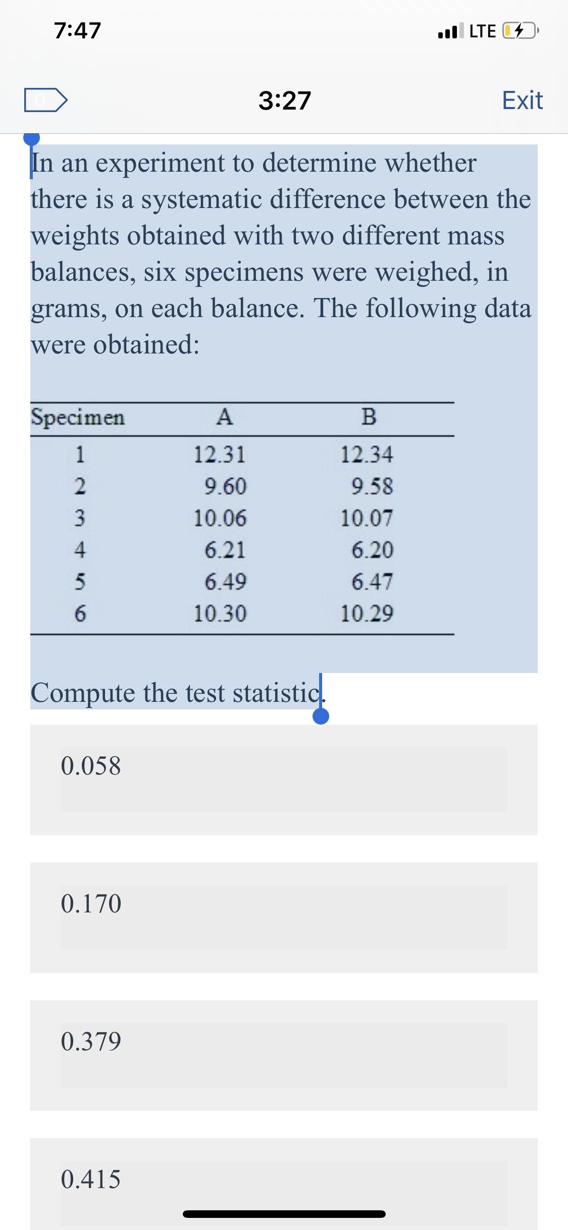
In an experiment to determine whether
there is a systematic difference between the
weights obtained with two different mass
balances, six specimens were weighed, in
grams, on each balance. The following data
were obtained:
Specimen
12.31
12.34
9.60
9.58
3
10.06
10.07
6.21
6.20
6.49
6.47
10.30
10.29
Compute the test statistic.
0.058
0.170
0.379
0.415
Expert Solution
This question has been solved!
Explore an expertly crafted, step-by-step solution for a thorough understanding of key concepts.
This is a popular solution
Trending nowThis is a popular solution!
Step by stepSolved in 2 steps with 1 images

Follow-up Questions
Read through expert solutions to related follow-up questions below.
Follow-up Question

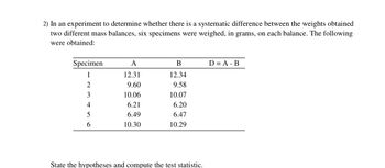
Transcribed Image Text:2) In an experiment to determine whether there is a systematic difference between the weights obtained
two different mass balances, six specimens were weighed, in grams, on each balance. The following
were obtained:
Specimen
1
2
3
4
5
6
A
12.31
9.60
10.06
6.21
6.49
10.30
B
12.34
9.58
10.07
6.20
6.47
10.29
State the hypotheses and compute the test statistic.
D = A - B
Solution
by Bartleby Expert
Follow-up Questions
Read through expert solutions to related follow-up questions below.
Follow-up Question

Transcribed Image Text:2) In an experiment to determine whether there is a systematic difference between the weights obtained
two different mass balances, six specimens were weighed, in grams, on each balance. The following
were obtained:
Specimen
1
2
3
4
5
6
A
12.31
9.60
10.06
6.21
6.49
10.30
B
12.34
9.58
10.07
6.20
6.47
10.29
State the hypotheses and compute the test statistic.
D = A - B
Solution
by Bartleby Expert
Knowledge Booster
Similar questions
- A sample of birth weights of 48 girls was taken. Below are the results (in g): 2724.5 3340.1 3243.6 3442.1 2996.9 3042 3505 3161.8 4022.8 3362.9 3768.9 2951.9 3229.7 2997.5 3758.1 3350.2 3210.7 3684.3 3530.1 3132.7 2776.9 3492.7 2655.1 3790.9 3064.6 3744.6 3294.5 2654.7 3536.6 2781.1 3756.3 3531.5 3654.2 3505.1 4018.6 3038 3202.3 3006 3701.6 3451.4 2986.5 3541.2 3232.9 2966 3186 3550.3 3056.6 3467.1 x = 3314.6 g s = 347.35 g Use a 5% significance level to test the claim that the standard deviation of birth weights of girls is less than the standard deviation of birth weights of boys, which is 530 g. Round all answers to 3 decimal places if possible. Procedure: Select an answer Step 1. Hypotheses Set-Up: %3D Ho: Select an answer На: Select an answer The test is a Select an answer O test. Step 2. The significance level is a = Step 3. Compute the value of the test statistic: Select an answer >arrow_forward--In an experiment to determine whether there is a systematic difference between the weights obtained with two different scales, 10 rock specimens were weighed, in grams, on each scale. The following data was obtained: 1 2 3 4 5 6 7 8 9 10 Weight on scale 1 11.14 15.38 8.33 10.30 23.44 9.13 13.46 6.44 12.51 19.35 Weight on scale 2 11.2 15.43 8.39 10.33 23.41 9.14 13.50 6.43 12.54 19.34 Construct a 96% confidence interval for the mean difference in weight between the two scales. Interpret the results. INTERPRET THE RESULTSarrow_forwardAn experimental diet to induce weight loss was followed for one week by a randomly selected group of 12 students with the following results. Loss in Pounds Student 1 2 3 5 6 7 8 9 10 11 12 2.5 2.9 0.4 1.7 0.0 1.5 5.5 3.5 3.9 3.5 1.1 2.9 (a) Find a point estimate for the average amount lost after one week on this diet. 2.55 ]x Is this an unbiased estimate of the population mean? Explain. Yes, this an unbiased estimate of the population mean, since E(X) = µ. Yes, this an unbiased estimate of the population mean, since E(X) + μ. O No, this is not an unbiased estimate of the population mean, since E(X) * μ. O No, this is not an unbiased estimate of the population mean, since E(X) = μ. O No, this is not an unbiased estimate of the population mean, since the sample size is too small. (b) Find a point estimate for the variance of the amount lost on this diet. (Round your answer to four decimal places.) 2.3264 x Is this an unbiased estimate of the population variance? Explain. Yes, this an…arrow_forward
- In an experiment to determine whether there is a systematic difference between the weights obtained with two different scales, 10 rock specimens were weighed, in grams, on each scale. The following data were obtained: Specimen Weight on Scale 1 Weight on Scale 2 1 13.36 13.19 2 16.80 16.43 3 9.75 9.52 4 11.03 11.47 5 26.00 26.22 6 10.80 10.73 7 14.68 14.74 8 6.60 6.72 9 13.02 12.95 10 22.29 22.64 Let μ1 represent the mean weight on Scale 1 and =μd−μ1μ2.Can you conclude that the the mean weight on Scale 1is less than the mean weight on Scale 2? Use the = α0.05 level of significance. (a) State the null and alternate hypotheses. (b) Compute the test statistic. (c) State a conclusion.arrow_forwardCalculate sdarrow_forwardFind the standardized test statistic t for a sample with n = 25, x = 12, s = 3, and a = 0.005 if Ho: μ = 11 Round your answer to three decimal places. 1.667 1.997 1.239 1.452arrow_forward
arrow_back_ios
arrow_forward_ios
Recommended textbooks for you
 MATLAB: An Introduction with ApplicationsStatisticsISBN:9781119256830Author:Amos GilatPublisher:John Wiley & Sons Inc
 Probability and Statistics for Engineering and th...StatisticsISBN:9781305251809Author:Jay L. DevorePublisher:Cengage Learning
 Statistics for The Behavioral Sciences (MindTap C...StatisticsISBN:9781305504912Author:Frederick J Gravetter, Larry B. WallnauPublisher:Cengage Learning
 Elementary Statistics: Picturing the World (7th E...StatisticsISBN:9780134683416Author:Ron Larson, Betsy FarberPublisher:PEARSON
 The Basic Practice of StatisticsStatisticsISBN:9781319042578Author:David S. Moore, William I. Notz, Michael A. FlignerPublisher:W. H. Freeman
 Introduction to the Practice of StatisticsStatisticsISBN:9781319013387Author:David S. Moore, George P. McCabe, Bruce A. CraigPublisher:W. H. Freeman

MATLAB: An Introduction with Applications
Statistics
ISBN:9781119256830
Author:Amos Gilat
Publisher:John Wiley & Sons Inc

Probability and Statistics for Engineering and th...
Statistics
ISBN:9781305251809
Author:Jay L. Devore
Publisher:Cengage Learning

Statistics for The Behavioral Sciences (MindTap C...
Statistics
ISBN:9781305504912
Author:Frederick J Gravetter, Larry B. Wallnau
Publisher:Cengage Learning

Elementary Statistics: Picturing the World (7th E...
Statistics
ISBN:9780134683416
Author:Ron Larson, Betsy Farber
Publisher:PEARSON

The Basic Practice of Statistics
Statistics
ISBN:9781319042578
Author:David S. Moore, William I. Notz, Michael A. Fligner
Publisher:W. H. Freeman

Introduction to the Practice of Statistics
Statistics
ISBN:9781319013387
Author:David S. Moore, George P. McCabe, Bruce A. Craig
Publisher:W. H. Freeman