
College Algebra
1st Edition
ISBN: 9781938168383
Author: Jay Abramson
Publisher: OpenStax
expand_more
expand_more
format_list_bulleted
Related questions
Question
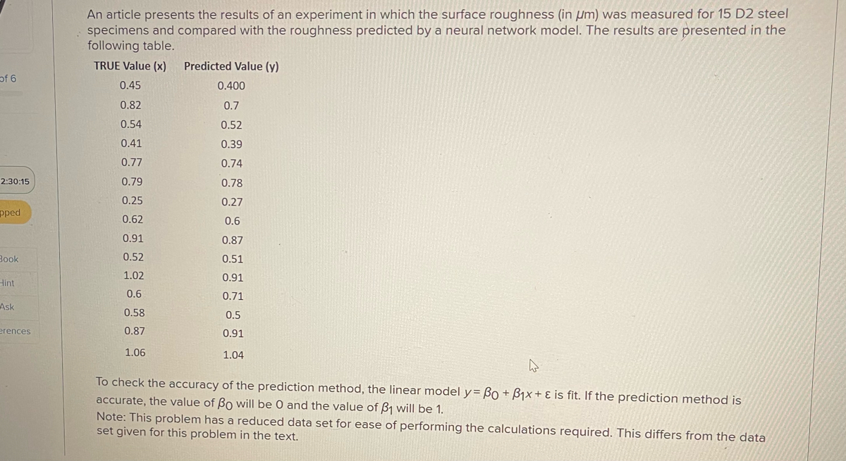

Transcribed Image Text:An article presents the results of an experiment in which the surface roughness (in μm) was measured for 15 D2 steel
specimens and compared with the roughness predicted by a neural network model. The results are presented in the
following table.
TRUE Value (x)
Predicted Value (y)
of 6
0.45
0.400
0.82
0.7
0.54
0.52
0.41
0.39
0.77
0.74
2:30:15
0.79
0.78
0.25
0.27
pped
0.62
0.6
0.91
0.87
0.52
Book
0.51
1.02
0.91
Hint
0.6
0.71
Ask
0.58
0.5
erences
0.87
0.91
1.06
1.04
۵
To check the accuracy of the prediction method, the linear model y=Bo+B1x+ & is fit. If the prediction method is
accurate, the value of Bo will be 0 and the value of ẞ1 will be 1.
Note: This problem has a reduced data set for ease of performing the calculations required. This differs from the data
set given for this problem in the text.
Expert Solution
This question has been solved!
Explore an expertly crafted, step-by-step solution for a thorough understanding of key concepts.

Step by stepSolved in 3 steps with 10 images

Knowledge Booster

Similar questions
- Lecture(8.8): The amount of time people engage in physical activity mat be related to health outcome. Those who report that they spend more than 15 hours are put into one while those who spend less 10 were put into another group. (Those who fall in between 10 and 15 were left out of the study); The reaearcher then ask the participants to wear a monitor for one month. The average time in minutes is recorded and shown below . Is there any evidence that on average people who watch less than 10 hours watching televsion spend more time on physical activity.?. Test the hypotheses at (alpha=0.05) using the 5 step procedure <10 hours 75 63 118 35 82 >15 hours 62 6 78 43 22 33arrow_forwardEXAMPLE 8.5 | Alloy Adhesion An article in the Journal of Materials Engineering ["Instrumented Tensile Adhesion Tests on Plasma Sprayed Thermal Barrier Coatings" (1989, Vol. 11(4), pp. 275-282)] describes the results of tensile adhesion tests on 22 U-700 alloy specimens. The load at specimen failure is as follows (in megapascals): 19.8 15.4 11.4 19.5 10.1 18.5 14.1 8.8 14.9 7.9 17.6 13.6 O 0.01 O 0.025 O 0.05 O 0.95 O 0.975 7.5 12.7 16.7 11.9 15.4 11.9 15.8 11.4 The sample mean is x = 13.71, and the sample standard deviation is s = 3.55. Figures 8.6 and 8.7 show a box plot and a normal probability plot of the tensile adhesion test data, respectively. These displays provide good support for the assumption that the population is normally distributed. We want to find a 95% CI on μ. Since n = 22, we have n - 1 = 21 degrees of freedom for t, so to.025,21 = 2.080. The resulting CI is X-1/2-1/√x+1a/2n-1³/√n 13.71-2.080 (3.55)/√/22 ≤ ≤ 13.71 +2.080 (3.55)/√22 13.711.57 ≤ ≤ 13.71 +1.57 12.14 ≤…arrow_forward6 A study was conducted that measured the total brain volume (TBV) (in mm3) of patients that had schizophrenia and patients that are considered normal. Table #1 contains the TBV of the normal patients and Table #2 contains the TBV of schizophrenia patients ("SOCR data Oct2009," 2013). Table #1: Total Brain Volume (in mm3) of Normal Patients 1663407 1583940 1299470 1535137 1431890 1578698 1453510 1650348 1288971 1366346 1326402 1503005 1474790 1317156 1441045 1463498 1650207 1523045 1441636 1432033 1420416 1480171 1360810 1410213 1574808 1502702 1203344 1319737 1688990 1292641 1512571 1635918 Table #2: Total Brain Volume (in mm3) of Schizophrenia Patients 1331777 1487886 1066075 1297327 1499983 1861991 1368378 1476891 1443775 1337827 1658258 1588132 1690182 1569413 1177002 1387893 1483763 1688950 1563593 1317885 1420249 1363859 1238979…arrow_forward
- The least-squares regression equation is y = 689.9x + 14,803 where y is the median income and x is the percentage of 25 years and older with at least a bachelor's degree in the region. The scatter diagram indicates a linear relation between the two variables with a correlation coefficient of 0.7256. Complete parts (a) through (d). (a) Predict the median income of a region in which 20% of adults 25 years and older have at least a bachelor's degree. (Round to the nearest dollar as needed.) . TOLED dian Income Media 55000- 20000- 15 20 25 30 35 40 45 50 55 60 Bachelor's 96 Qarrow_forwardA coffee shop owner offers two brands of coffee, Brand "A" and Brand "B". The proportion of clients that prefer Brand "A" is 60%. Recently, the price of Brand "A" went up. The proportion of clients that buy brand "A" among the first 15 customers that enter the shop after the change in price is an estimator of the current proportion of clients that prefer Brand "A". Assume that the change in price has no effect on the preference of the clients. Then the mean squared error (MSE) of the estimator is equal to: (Give an answer of the form x.xxx, i.e. with 3 significance digits) (HINT: Carefully read the definition of MSE in Chapter 10 of the text book.)arrow_forwardSuppose that you wish to estimate the effect of class attendance on student performance. A basic model is examscore = β0 + β1attendance + β2priorGP A + u where examscore is students’ score on the exam (from 1 to 6), attendance is the number of TA sessions attended on Zoom (from 0 to 9), and priorGPA is the average exam grade last year. (a) Let internet be the quality of internet at the student’s study place. Do you think internet satisfies the independence assumption? What about the exclusion restriction? (b) Assuming that internet satisfies the conditions above, what other condition must internet satisfy in order to be a valid IV for attendance? (c) Suppose, we add the interaction term priorGP A × attendance. Interpret the coefficient on the interaction term. (d) (Difficult) If attendance is endogenous, then, in general, so is priorGP A × attendance. What might be a good IV for priorGP A × attendance?arrow_forward
- Explain the Stationarity in the AR(1) Model?arrow_forwardshow workarrow_forwardConsider a single variable model to estimate the effect of in-person lecture attendance on university students' WAMs (weighted average marks): (C1) WAM = β0 + β1Attend + u Where: WAMis a student's weight average mark Attendis the proportion of lectures attended by a student in an academic year Using the information above, answer the following 3 questions. [i] Explain why Attend might be endogenous in Model (C1). What does this suggest about E [u ∣ Attend]? [ii] Suppose that student attendance is related to a student's conscientiousness. Does this mean that conscientiousness would be a good instrumental variable for Attend? Why or why not? Explain your reasoning. [iii] Unfortunately a major strike by railway works disrupts transport links to 3 of the 7 universities in a city for a period of 2 weeks. This temporarily means that students who are enrolled at those 3 affected universities cannot attend lectures in person. Carefully explain how you would use this information to…arrow_forward
- 6B A study was conducted that measured the total brain volume (TBV) (in mm3) of patients that had schizophrenia and patients that are considered normal. Table #1 contains the TBV of the normal patients and Table #2 contains the TBV of schizophrenia patients ("SOCR data Oct2009," 2013). Table #1: Total Brain Volume (in mm3) of Normal Patients 1663407 1583940 1299470 1535137 1431890 1578698 1453510 1650348 1288971 1366346 1326402 1503005 1474790 1317156 1441045 1463498 1650207 1523045 1441636 1432033 1420416 1480171 1360810 1410213 1574808 1502702 1203344 1319737 1688990 1292641 1512571 1635918 Table #2: Total Brain Volume (in mm3) of Schizophrenia Patients 1331777 1487886 1066075 1297327 1499983 1861991 1368378 1476891 1443775 1337827 1658258 1588132 1690182 1569413 1177002 1387893 1483763 1688950 1563593 1317885 1420249 1363859 1238979…arrow_forwardIn Exercise 7.25, we saw data from Everitt that showed that girls receiving cognitive behavior therapy gained weight over the course of that therapy. However, it is possible that they just gained weight because they got older. One way to control for this is to look at the amount of weight gained by the cognitive therapy group (n = 29) in contrast with the amount gained by girls in a Control group (n = 26), who received no therapy. The data on weight gain for the two groups is shown below. Control Cognitive Therapy -0.5 3.3 1.7 -9.1 -9.3 11.3 0.7 2.1 -5.4 0.0 -0.1 -1.4 12.3 -1.0 -0.7 1.4 -2.0 - 10.6 -3.5 -0.3 -3.7 - 10.2 - 12.2 -4.6 14.9 -6.7 3.5 -0.8 11.6 2.8 17.1 2.4 -7.1 0.3 -7.6 12.6 6.2 -0.2 1.8 1.6 1.9 3.7 11.7 3.9 -9.2 15.9 6.1 0.1 8.3 - 10.2 1.1 15.4 -4.0 -0.7 20.9 Мean -0.45 3.01 St Dev. 7.99 7.31 Variance 63.82 53.41 Run the appropriate test to compare the group means. What would you conclude?arrow_forwardThe least-squares regression equation is y = 758.4x + 12.9 12,935 where y is the median income and is the percentage of 25 years and older with at least a bachelor's degree in the region. The scatter diagram indicates a linear relation between the two variables with a correlation coefficient of 0.7500. (a) Predict the median income of a region in which 30% of adults 25 years and older have at least a bachelor's degree.arrow_forward
arrow_back_ios
SEE MORE QUESTIONS
arrow_forward_ios
Recommended textbooks for you
 Linear Algebra: A Modern IntroductionAlgebraISBN:9781285463247Author:David PoolePublisher:Cengage Learning
 Big Ideas Math A Bridge To Success Algebra 1: Stu...AlgebraISBN:9781680331141Author:HOUGHTON MIFFLIN HARCOURTPublisher:Houghton Mifflin Harcourt
 Glencoe Algebra 1, Student Edition, 9780079039897...AlgebraISBN:9780079039897Author:CarterPublisher:McGraw Hill
 Elementary Linear Algebra (MindTap Course List)AlgebraISBN:9781305658004Author:Ron LarsonPublisher:Cengage Learning
Linear Algebra: A Modern Introduction
Algebra
ISBN:9781285463247
Author:David Poole
Publisher:Cengage Learning
Big Ideas Math A Bridge To Success Algebra 1: Stu...
Algebra
ISBN:9781680331141
Author:HOUGHTON MIFFLIN HARCOURT
Publisher:Houghton Mifflin Harcourt
Glencoe Algebra 1, Student Edition, 9780079039897...
Algebra
ISBN:9780079039897
Author:Carter
Publisher:McGraw Hill
Elementary Linear Algebra (MindTap Course List)
Algebra
ISBN:9781305658004
Author:Ron Larson
Publisher:Cengage Learning