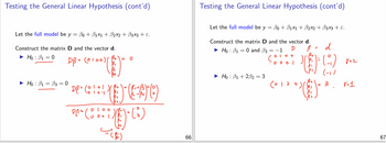
Testing the General Linear Hypothesis (cont'd)Let the full model be y = ẞ0 + ẞ1×1 + ẞ2x2 + ẞ3x3 + ε.Construct the matrix D and the vector d.Hoẞ1 = 0► Hoẞ1 = ẞ3 = 0DB = (0100)/(༠ ༩༠༠)(DP = (010-1DA² Coo000= 0DEAO=(i)Testing the General Linear Hypothesis (cont'd)Let the full model be y = ẞ0 + ẞ1×1 + ẞ2×2 + B3x3 + ε.Construct the matrix D and the vector d.► Hoẞ1 = 0 and ẞ3= −1DHoẞ1+2ẞ2 = 30100·00016012ام=Ο=d()822(-1)38=1996667 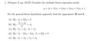1. (Chapter 3, pp. 65-67) Consider the multiple linear regression modely = ßo + ß1x1 + ẞ2x2 + ẞ3x3 + ß4×4 + ɛ.For the general linear hypothesis approach, find the appropriate D and d.(a) Hoẞ1+2ẞ₂ = 3B1 + B2(b) Ho:= ẞ32(c) Ho B1 B2, B3 = ẞ4=(d) Hoẞ12ẞ2 = 4ẞ3, ẞ1 +2ẞ2 = 0(e) Hoẞ₁ = B₂ = ß3 = ß4

The given multiple linear regression model is as follows.

Answered: 1. (Chapter 3, pp. 65-67) Consider the…

MATLAB: An Introduction with Applications

6th Edition

ISBN:9781119256830

Author:Amos Gilat

Publisher:Amos Gilat

Chapter1: Starting With Matlab

Section: Chapter Questions

Problem 1P

See similar textbooks

Similar questions

A property agent wants to study the relationship between the age of a house (X) and its selling price (Y). Listed below is a random sample of houses that the agent has sold recently. [House] [Age in Years (X)] [Selling Price in $'m (Y)] 1 9 2.2 2 7 1.9 3 11 1.7 4 12 0.8 5 8 2.5 a) Determine the linear regression equation. b) i. If the age of a house is 10 year-old, what is the selling price? ii. If the age of a house is 20 year-old, what is the selling price? c) i. Determine the correlation coefficient. ii. Interpret the result.
The Simple Linear Regression model is Y = b0 + b1*X1 + u and the Multiple Linear Regression model with k variables is: Y = b0 + b1*X1 + b2*X2 + ... + bk*Xk + u Y is the dependent variable, the X1, X2, ..., Xk are the explanatory variables, b0 is the intercept, b1, b2, ..., bk are the slope coefficients, and u is the error term, Yhat represents the OLS fitted values, uhat represent the OLS residuals, b0_hat represents the OLS estimated intercept, and b1_hat, b2_hat,..., bk_hat, represent the OLS estimated slope coefficients. QUESTION 13 In the MLR model, what do we mean by Heteroskedasticity? That the error term depends on the values of the explanatory variables That all the explanatory variables have different variance That the variance of the error term is a function of the explanatory variables That the variance of the error term is constant QUESTION 14 Suppose that in the model Y=b0+b1*X1+u, we add a variable that is correlated with both Y and X1. What will happen…
An owner of a home in the Midwest installed solar panels to reduce heating costs. After installing the solar panels, he measured the amount of natural gas used y (in cubic feet) to heat the home and outside temperature x (in degree-days, where a day's degree-days are the number of degrees its average temperature falls below 65° F) over a 23-month period. He then computed the least-squares regression line for predicting y from x and found it to be ŷ = 85 + 16x. The software used to compute the least-squares regression line for the equation above says that r2 = 0.98. This suggests which of the following? 1. Gas used increases by square root of 0.98 = 0.99 cubic feet for each additional degree-day? 2. Although degree-days and gas used are correlated, degree-days do not predict gas used very accurately. 3. Prediction of gas used from degree-days will be quite accurate.
7
Find the equation y = Bo + B₁x of the least-squares line that best fits the given data points. (1,3), (2,3), (3,4), (4,4) The line is y = 2.49 + 0.44 x. (Type integers or decimals.)
Can you answer the questions in 3b, 3c, and 3d? Thank you
An engineer wants to determine how the weight of a gas-powered car, x, affects gas mileage, y. The accompanying data represent the weights of various domestic cars and their miles per gallon in the city for the most recent model year. Complete parts (a) through (d) below. (a) Find the least-squares regression line treating weight as the explanatory variable and miles per gallon as the response variable. y=nothingx+(nothing) (Round the x coefficient to five decimal places as needed. Round the constant to one decimal place as needed.) (b) Interpret the slope and y-intercept, if appropriate. Choose the correct answer below and fill in any answer boxes in your choice. (Use the answer from part a to find this answer.) A. A weightless car will get nothing miles per gallon, on average. It is not appropriate to interpret the slope. B. For every pound added to the weight of the car, gas mileage in the city will decrease by nothing mile(s) per gallon, on…
The Simple Linear Regression model is Y = b0 + b1*X1 + u and the Multiple Linear Regression model with k variables is: Y = b0 + b1*X1 + b2*X2 + ... + bk*Xk + u Y is the dependent variable, the X1, X2, ..., Xk are the explanatory variables, b0 is the intercept, b1, b2, ..., bk are the slope coefficients, and u is the error term, Yhat represents the OLS fitted values, uhat represent the OLS residuals, b0_hat represents the OLS estimated intercept, and b1_hat, b2_hat,..., bk_hat, represent the OLS estimated slope coefficients. QUESTION 4 Suppose we have an SLR model, where the dependent variable (Y) represents ‘how satisfied someone is with his/her life, from 0 to 100’ (the higher the value, the higher the satisfaction with life), and the explanatory variable (X1) represents ‘personal annual income in £1,000’. The estimated OLS regression line is: Yhat = 33.2 + 0.74*X1. According to this model, what is the predicted life satisfaction, for someone with…
q7-
Suppose you want to test whether X2 and X3 can jointly explain Y in the following regression model: Y = Bo + B1X1 + B,X2 + B3X3 + u You obtain data for 85 observations and conduct a joint test of significance at 1% level. Your restricted model is given by, OY = Bo + B3X3 +u OY = Bo + B1X1 + B3 X3 + u OY = Bo + B1X1 + u OY = Bo + u
A set of experimental runs were made to determine a way of predicting a parameter Z in terms of A and B. The results are represented in TABLE 1. 1) Using simple linear regression models, find the missing values in TABLE 1. 2) Using TWO (2) different methods, determine which independent variable is the most linearly related to the dependent variable? Show your calculations and discuss your results. 3) Using a multiple linear regression model, find the missing values in TABLE 1. Compare your results with those obtained in question 1) and discuss your findings. 4) Analyze and discuss the fitness of the multiple linear regression model for the data. TABLE 1. Z 22.1 12 16.5 17.9 7.2 11.8 9.2 19 22.4 12.5 24.4 11.3 14.6 18 20.9 18.9 A 37.8 45.9 a₁ 10.8 48.9 32.8 B 69.2 69.3 58.5 58.4 75 23.5 65.9 46 52.9 b₁ 55.8 18.3 19.1 53.4 22.9 22.9 a2 32.9 47.7 36.6 39.6 20.5 23.9 27.7 16.7 27.1 **The End*
The Simple Linear Regression model is Y = b0 + b1*X1 + u and the Multiple Linear Regression model with k variables is: Y = b0 + b1*X1 + b2*X2 + ... + bk*Xk + u Y is the dependent variable, the X1, X2, ..., Xk are the explanatory variables, b0 is the intercept, b1, b2, ..., bk are the slope coefficients, and u is the error term, Yhat represents the OLS fitted values, uhat represent the OLS residuals, b0_hat represents the OLS estimated intercept, and b1_hat, b2_hat,..., bk_hat, represent the OLS estimated slope coefficients. QUESTION 28 Suppose your estimated MLR model is: Y_hat = -30 + 2*X1 + 10*X2 Suppose the standard error for the estimated coefficient associated with X2 is equal to 5. Now, suppose that for some reason we multiply X2 by 5 and we re-estimate the model using the rescaled explanatory variable. What will be the value of the estimated coefficient of X2 and its standard error? The estimated coefficient of X2 will be equal to 50 and its standard error will be…

SEE MORE QUESTIONS

Recommended textbooks for you

MATLAB: An Introduction with Applications

Statistics

ISBN:

9781119256830

Author:

Amos Gilat

Publisher:

John Wiley & Sons Inc

Probability and Statistics for Engineering and th…

Statistics

ISBN:

9781305251809

Author:

Jay L. Devore

Publisher:

Cengage Learning

Statistics for The Behavioral Sciences (MindTap C…

Statistics

ISBN:

9781305504912

Author:

Frederick J Gravetter, Larry B. Wallnau

Publisher:

Cengage Learning

MATLAB: An Introduction with Applications

Statistics

ISBN:

9781119256830

Author:

Amos Gilat

Publisher:

John Wiley & Sons Inc

Probability and Statistics for Engineering and th…

Statistics

ISBN:

9781305251809

Author:

Jay L. Devore

Publisher:

Cengage Learning

Statistics for The Behavioral Sciences (MindTap C…

Statistics

ISBN:

9781305504912

Author:

Frederick J Gravetter, Larry B. Wallnau

Publisher:

Cengage Learning

Elementary Statistics: Picturing the World (7th E…

Statistics

ISBN:

9780134683416

Author:

Ron Larson, Betsy Farber

Publisher:

PEARSON

The Basic Practice of Statistics

Statistics

ISBN:

9781319042578

Author:

David S. Moore, William I. Notz, Michael A. Fligner

Publisher:

W. H. Freeman

Introduction to the Practice of Statistics

Statistics

ISBN:

9781319013387

Author:

David S. Moore, George P. McCabe, Bruce A. Craig

Publisher:

W. H. Freeman

SEE MORE TEXTBOOKS