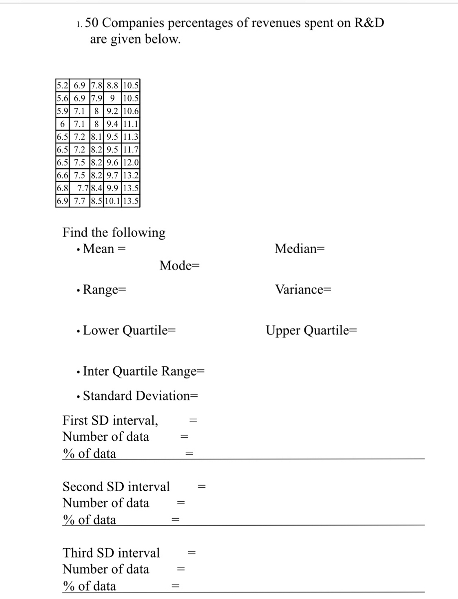
1. 50 Companies percentages of revenues spent on R&D are given below. 5.2 6.9 7.8 8.8 10.5 5.6 6.9 7.9 9 10.5 5.9 7.1 8 9.2 |10.6 6 7.1 89.4 11.1 |6.5 7.2 8.1 9.5 |11.3 6.5 7.2 8.2 9.5 11.7 6.5 7.5 8.2 9.6 |12.0 6.6 7.5 8.2 9.7 |13.2 |6.8 7.78.4 9.9 13.5 6.9 7.7 8.5 10.1|13.5 Find the following • Mean = Median= Mode= • Range= Variance= • Lower Quartile= Upper Quartile= • Inter Quartile Range= • Standard Deviation= First SD interval, Number of data % of data Second SD interval Number of data % of data Third SD interval Number of data % of data

5. The graph below shows the LFPR for 25-54 year old men over several decades. Percent 100 May-16 98 96 94 92 90 88 86 1948 1954 1960 1966 1972 1978 1984 1990 1996 2002 2008 2014 Source: Bureau of Labor Statistics, Current Population Survey; CEA calculations. (Source: Voxeu.org) It shows that the fraction of these "prime working age men" who are NOT in the labor forced has a. doubled b. tripled c. quadrupled d. not changed

All companies are rightly concerned about the income disparity between Males and Females and FringeTech is no different. Is there any evidence in the data that Males are earning more than Females on average? Gender Income ($000) F 94.1 F 69.4 F 81.7 F 72.1 F 90.1 F 84.4 F 77.5 F 124 F 71.2 F 72.1 F 75.7 F 79.8 F 76.7 F 65.1 F 83.8 F 85.8 F 70.6 F 93.3 F 80.1 F 80.8 F 85.5 F 62.1 F 88.5 F 88.2 F 110.3 F 124.6 F 97.6 F 82.4 F 58.2 F 75.5 F 75.1 F 70.5 F 83.9 F 95.5 F 150.2 F 84.4 F 88.7 F 135.4 F 72.3 F 65.5 F 80.3 F 136.8 F 75.8 F 47.5 F 86.6 F 64.4 F 99.3 F 40 F 69.1 F 107.7 F 74.7 F 90.3 F 82.2 F 97 F 125.3 F 111.1 F 60.4 F 102.7 F 89 F 69.4 F 61.6 F 93.1 F 87.2 F 67.7 F 130.6 F 83.2 F 50.4 F 132.7 F 69.1 F 103.6 F 80.2 F 73.9 F 56.3 F 130.2 F 80.7 M 83.1 M 95.4 M 128.2 M 127.3 M 96.8 M 94 M 125.5 M 107.2 M 92.4 M…

Mag    Depth 2.96     19.9 2.73     6.5 1.46     3.5 0.85     13.3 2.95     19.9 1.63     8.7 1.92     18.4 1.12     7.9 2.59     3.1 1.68     9.4 0.14     6.2 2.43     17.7 0.04     18.4 1.03     9.8 2.89     12.4 0.54     9.5 0.77     2.1 1.87     8.1 2.72     17.3 0.84     9.9 1.48     12.7 0.68     7.1 1.83     17.1 1.89     3.4 0.94     13.8 2.24     5.7 0.94     16.7 1.36     5.2 0.98     6.6 0.51     12.5 2.69     14.1 1.73     12.5 2.29     12.7 1.63     14.7 0.52     18.6 2.75     4.5 2.31     10.5 1.39     13.3 2.05     10.5 0.63     5.7 1.15     3.6 1.59     2.9 2.92     11.3 0.33     6.4 2.78     9.2 1.43     4.8 0.82     4.8 0.21     13.6 1.77     12.3 0.68     4.9 1) Check Image 2) Given that the earthquake has a magnitude of 1.1, the best predicted depth is     km. ​(Round to one decimal place as​ needed.)

The table shows the annual compensation of 40 randomly chosen CEOs (millions of dollars).  4.93 1.93 24.16 10.10 13.76 6.28 3.28 4.61 192.38 17.25 25.53 8.92 12.48 18.24 1.80 6.58 67.86 13.97 27.34 4.45 11.50 4.41 2.27 6.22 26.20 14.43 18.61 4.64 9.42 3.23 0.88 3.56 31.07 12.81 23.59 6.59 8.74 4.25 1.38 2.22 (b) Describe the shape of the histogram. A) The distribution is skewed to the left. B) The distribution is symmetric. C) The distribution is skewed to the right   (c) Identify any unusual values. (Round your answers to 2 decimal places.)     Unusual values   million   million

The number of adult Americans who smoke continues to drop. The table contains estimates of the percentages of adults (ages 1818 and over) who were smokers in the years between 1965 and 201715.and 201715. ???? ?Year � ??????? ?Smokers � 1965 41.94 1970 37.4 1974 37.1 1978 34.1 1980 33.2 1983 32.1 1985 30.1 1987 28.8 1990 25.5 1993 25.0 1995 24.7 1997 24.7 1999 23.5 2001 22.8 2002 22.5 2004 20.9 2006 20.8 2008 20.6 2010 19.3 2012 18.1 2014 16.8 2017 14.0   According to your regression line, how much did smoking decline per year during this period, on the average? Give your answer to three decimal places. average smoking decline:   percentage points

214.26 356.79 424.96 231.51 353.89 552.75 281.93 303.66 518.15 234.62 336.36 514.07 246.55 341.26 575.65 277.97 452.59 652.23 267.33 482.71 775.82 209.67 445.44 769.54 372.05 428.84 765.86 320.02 485.78 819.89.  The table below contains the total cost​ ($) for four tickets to a basketball game purchased on the secondary​ market, two​ beers, two soft​ drinks, two hot​ dogs, and one parking space at each arena during a recent season.   a. Organize these costs as an ordered array. b. Construct a frequency distribution and a percentage distribution for these costs. c. Around what​ values, if​ any, are at least​ 75% of the costs of attending the game​ concentrated? Explain. Question content area bottom Part 1 a. Organize these costs as an ordered array.    enter your response here    enter your response here    enter your response here    enter your response here    enter your response here    enter your response here    enter your response here    enter your response here    enter your…

Hours Spent in Child Care 5.5 11.4 2.1 11.0 7.2 5.1 9.1 10.2 2.9 8.7 10.0 9.0 9.8 9.4 3.1 8.5 9.6 10.6 7.6 8.9 10.7 6.0 0.6 3.7 9.8 3.3 3.5 5.0 3.3 10.3 7.3 6.9 6.1 4.3 0.8 6.9 8.1 1.3 1.6 9.8   Sample Size 40                     Hypothesized Mean 6

2. This table shows the mean and median total cash income for married-couple households (including wages, public assistance, interest/dividends, Social Security, pensions, etc.), by race and Hispanic origin. a apaa Median Household Mean Household Income ($) Income ($) Asian 110,453 78,010 66,893 110,138 145,948 Black 97,667 Hispanic White, non-Hispanic 88,450 129,142 a. Pick one group and interpret the median and the mean. b. For each group, how do the mean and the median compare? Explain why you think this must be the case.

First Die 4 6. 1 3 4 6. 7 3 4 5. 6. 7. 8. 4 5. 6. 7 8. 9. 4 6. 7. 8. 9. 10 5 6. 8 6. 10 11 8. 9. 10 11 12 419 t in 47 Second Die