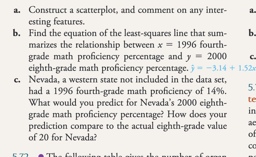
Construct a scatterplot, and comment on any inter- esting features. a. b. C. b. Find the equation of the least-squares line that sum- marizes the relationship between x = 1996 fourth- grade math proficiency percentage and y = 2000 eighth-grade math proficiency percentage. ŷ = −3.14 + 1.52x c. Nevada, a western state not included in the data set, had a 1996 fourth-grade math proficiency of 14%. What would you predict for Nevada's 2000 eighth- grade math proficiency percentage? How does your prediction compare to the actual eighth-grade value of 20 for Nevada? 5. te in ae of CO 5.72 numba 08x 5.71 Percentages of public school students in fourth grade in 1996 and in eighth grade in 2000 who were at or above the proficient level in mathematics were given in the article "Mixed Progress in Math" (USA Today, August 3, 2001) for eight western states: State 4th grade (1996) 8th grade (2000) Arizona 15 21 California 11 18 Hawaii 16 16 Montana 22 37 New Mexico Oregon Utah Wyoming 2232 19 13 13 21 32 225 26

A recent study on driving behavior examined whether the combination of high driving skills and low safety skills is dangerous. Participants were classified as high or low in driving skill based on responses to a driver-skill inventory, then classified as high or low in safety skill based on responses to a driver-aggression scale. An overall measure of driving risk was obtained by combining several variables such as number of accidents, tickets, tendency to speed, etc. The following data were obtained. Use a 2 x 2 ANOVA with the .05 significance level to evaluate the results. What cutoff score(s) should be used? Driving Skill Low High Safety Skill Low M1=5 M2=4.5 S1=2.7 S2=3.8 N1=6 N2=6 HIgh M3=3 M4=3.5 S3=2.9 S4=2.5 N3=6 N4=6 Group of answer choices +4.35 +3.40 +3.49 +4.26

fill blanks underlines.

4. Draw a line / curve of best fit for the following sets of data & identify if they are linear, quadratic or exponential: 2500 1500 1000 500 300 200 -100 25 50

Logging activity in forests is thought to affect the behavior of black bears. An important measure of animal behavior is the home range, the area used by animals in their daily lives. In a study of black bears in a logged Canadian forest, the spring and early summer home ranges (in square kilometers) of 12 radio-collared female black bears was measured. The results are below. Assume the home range of female black bears in this logged forest is normally distributed. 39.9, 23.5, 42.1, 29.4, 34.4, 40.9, 27.9, 22.3, 13.0, 20.1, 13.3, 8.6 d) Construct and interpret a 95% confidence interval for the mean home range of female black bears in this logged forest. e) The typical home range of females in forests with no logging is 20 square kilometers. Based on the confidence interval above, do you think that the mean home range size of females in this logged forest could be the same as the mean home range size in non-logged forests? Explain.

A psychologist would like to examine the effects of caffeine consumption on the activity level of preschool children. Three samples of children are selected with n = 5 in each sample. One group gets no caffeine, one group gets a small dose, and the third group gets a large dose. The psychologist records the activity level for each child during 50 minutes of unstructured play. Determine whether these data indicate significant differences among the three groups using a = .05. Your answer should include hypotheses, critical boundary, F-score, and results including notation, decision, and explanation. Calculate and interpret effect size if appropriate. Indicate whether post- hoc test results should be calculated (i.e., "yes, include" or "no, do not include"). No caffeine Small dose Large dose T= 15 T= 20 T= 25 G = 60 SS = 16 SS = 12 SS = 20 Ex2 = 298

An athletic director proudly states that he has used the average GPAs of the university's sports teams and is predicting a high graduation rate for the teams. Why is this method unsafe? Choose the correct answer below. OA. This method is unsafe because the average GPA may differ for each team. Using the average of the average GPA of each team obscures the possibility that certain teams tend to perform less well in classes. B. This method is unsafe because there is more variation in the GPAs of the athletes than the average GPA of the university's sports teams. Strong students may offset weak students in calculating the average GPAS, which makes it appear more likely that most students are doing well. OC. This method is unsafe because it is dangerous to extrapolate into the future. Classes in university tend to become more difficult, which makes it less likely that the average GPA will hold as time goes on. D. This method is unsafe because there is a minimum GPA required to graduate. If…

A recent study on driving behavior examined whether the combination of high driving skills and low safety skills is dangerous. Participants were classified as high or low in driving skill based on responses to a driver-skill inventory, then classified as high or low in safety skill based on responses to a driver-aggression scale. An overall measure of driving risk was obtained by combining several variables such as number of accidents, tickets, tendency to speed, etc. The following data were obtained. Use a 2 x 2 ANOVA with the .05 significance level to evaluate the results. Which of the following is one of the research hypotheses? Driving Skill Low High Safety Skill Low M1=5 M2=4.5 S1=2.7 S2=3.8 N1=6 N2=6 HIgh M3=3 M4=3.5 S3=2.9 S4=2.5 N3=6 N4=6 Group of answer choices The difference in driving risk between drivers with high and low driving safety does not depend on driving skill level On average, drivers classified as high and low in safety skill do not…

Swifty produces 5-foot USB cables. During the past year, the company purchased 215,000 feet of plastic-coated wire at a price of $0.40 per foot. The direct materials standard for the cables allows 6 feet of wire at a standard price of $0.45 per foot. During the year, the company used a total of 245,000 feet of wire to produce 42,000 5-foot cables.Calculate Swifty’s direct materials quantity variance for the year. Direct material quantity variance   $        Is this favorable or not?