Concept explainers
Videos
Break into small groups and discuss the following topics. Organize a brief outline in which you summarize the main points of your group discussion.
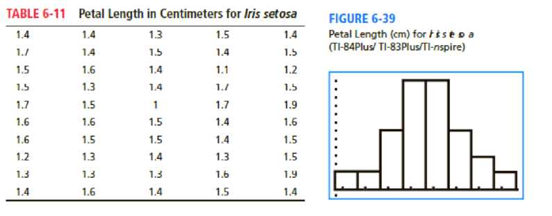
Iris setosa is a beautiful wildflower that is found in such diverse places as Alaska, the Gulf of St. Lawrence, much of North America, and even in English meadows and parks. R. A. Fisher, with his colleague Dr. Edgar Anderson, studied these flowers extensively. Dr. Anderson described how he collected information on irises:
I have studied such irises as I could get to see, in as great detail as possible, measuring iris standard after iris standard and iris fall after iris fall, sitting squat-legged with record book and ruler in mountain meadows, in cypress swamps, on lake beaches, and in English parks. [E. Anderson, “The Irises of the Gaspé Peninsula,” Bulletin, American Iris Society, Vol. 59 pp. 2–5, 1935.]
The data in Table 6-11 were collected by Dr. Anderson and were published by his friend and colleague R. A. Fisher in a paper titled “The Use of Multiple Measurements in Taxonomic Problems” (Annals of Eugenics, part II, pp. 179–188, 1936). To find these data, visit the Carnegie Mellon University Data and Story Library (DASL) web site. From the DASL site, look under Biology and Wild iris select Fisher's Irises Story.
Let x be a random variable representing petal length. Using a TI-84Plus/ TI-83Plus/TI-nspire calculator, it was found that the sample mean is
- (a) Examine the histogram for petal lengths. Would you say that the distribution is approximately mound-shaped and symmetric? Our sample has only 50 irises; if many thousands of irises had been used, do you think the distribution would look even more like a normal curve? Let x be the petal length of Iris setosa. Research has shown that x has an approximately
normal distribution , with mean μ = 1.5 cm and standard deviation σ = 0.2 cm. - (b) Use the
empirical rule with μ = 1.5 and σ = 0.2 to get an interval into which approximately 68% of the petal lengths will fall. Repeat this for 95% and 99.7%. Examine the raw data and compute the percentage of the raw data that actually fall into each of these intervals (the 68% interval, the 95% interval, and the 99.7% interval). Compare your computed percentages with those given by the empirical rule. - (c) Compute the
probability that a petal length is between 1.3 and 1.6 cm. Compute the probability that a petal length is greater than 1.6 cm. - (d) Suppose that a random sample of 30 irises is obtained. Compute the probability that the average petal length for this sample is between 1.3 and 1.6 cm. Compute the probability that the average petal length is greater than 1.6 cm.
- (e) Compare your answers to parts (c) and (d). Do you notice any differences? Why would these differences occur?
(a)
Explain whether the distribution is approximately mound-shaped and symmetrical.
Answer to Problem 1DH
Yes, the distribution is approximately mound-shaped and symmetrical.
Explanation of Solution
From the histogram for petal lengths, the distribution is approximately bell-shaped or mound-shaped and symmetrical because approximately the left half of the graph is the mirror image of the right half of the graph.
Our sample has only 50 irises; if many thousands of irises had been used, the distribution would look more similar to a normal curve because the sample is very large and the distribution of the sample will be approximately normally distributed.
(b)
Obtain the 68%, 95%, and 99% interval and compare the computed percentages with those given by the empirical rule.
Answer to Problem 1DH
The 68%, 95%, and 99% intervals are (1.3, 1.7), (1.1, 1.9), and (0.9, 2.1), respectively.
Explanation of Solution
Let x be the petal length of Iris Setosa and x has an approximately normal distribution, with mean
It is known that 68% of the observations will fall within one standard deviation of mean.
The 68% interval is as follows:
The 95% of the observations will fall within two standard deviations of mean.
The 95% interval is as follows:
The 99.7% of the observations will fall within two standard deviations of mean.
The 99.7% interval is as follows:
The 33 observations fall within the intervals 1.3 and 1.7;thus, the percentage of data within the intervals 1.3 and 1.7 is
The 46 observations fall within the intervals 1.1 and 1.9;thus, the percentage of data within the intervals 1.3 and 1.7 is
All data values fall within the intervals 0.9 and 2.1;thus, the percentage of data within the intervals 1.3 and 1.7 is
(c)
Obtain the probability that a petal length is between 1.3 and 1.6 cm and the probability that a petal length is greater than 1.6 cm.
Answer to Problem 1DH
The probability that a petal length is between 1.3 and 1.6 cm is 0.5328.
The probability that a petal length is greater than 1.6 cm is 0.3085.
Explanation of Solution
Let x be the petal length of Iris Setosa and x has an approximately normal distribution, with mean
The interval
The z-score for
The z-score for
The probabilitythat a petal length is between 1.3 and 1.6 cm is obtained as shown below:
In Appendix II, Table 5: Areas of a Standard Normal Distribution.
The values of
The probability corresponding to 0.5 is 0.6915 and the probability corresponding to -1 is 0.1587.
Hence, the probability that a petal length is between 1.3 and 1.6 cm is 0.5328.
The z-score for
The probability that a petal length is greater than 1.6 cm is obtained as given below:
Using Table 5 from the Appendix, the probability corresponding to 0.5 is 0.6915.
Hence, the probability that a petal length is greater than 1.6 cm is 0.3085.
(d)
Obtain the probability that the average petal length is between 1.3 and 1.6 cm and the probability that the average petal length is greater than 1.6 cm.
Answer to Problem 1DH
The probability that the average petal length is between 1.3 and 1.6 cm is 0.9972.
The probability that the averagepetal length is greater than 1.6 cm is 0.0027.
Explanation of Solution
Let x be the petal length of Iris Setosa and x has an approximately normal distribution, with mean
With sample size as n = 30, the sampling distribution for
The interval
The z-score for
The z-score for
The probability that the average petal length is between 1.3 and 1.6 cm is obtained as shown below:
In Appendix II, Table 5: Areas of a Standard Normal Distribution.
The values of
The probability corresponding to 2.78 is 0.9973 and the probability corresponding to -5.55does exist; Thus, it is considered as 0.0001.
Hence, the probability that the average petal length is between 1.3 and 1.6 cm is 0.9972.
The z-score for
The probability that the average petal length is greater than 1.6 cm is obtained as given below:
Using Table 5 from the Appendix, the probability corresponding to 2.78 is 0.9973.
Hence, the probability that the average petal length is greater than 1.6 cm is 0.0027.
(e)
Compare the results of Part (c) and Part (d); also delineate the differences.
Answer to Problem 1DH
The standard deviation of the sample mean is much smaller than the population standard deviation.
Explanation of Solution
In Part (c), x has a distribution that is approximately normal with
In Part (d),
The central limit theorem tells us that the standard deviation of the sample mean is much smaller than the population standard deviation.
Want to see more full solutions like this?
Chapter 6 Solutions
Understandable Statistics: Concepts and Methods


- Which of the following is not correct about diagram? O a. Requires drawing skill O b. Depict categorical and geographic data O c. Drawn on plain paper O d. Furnish more accurate informationarrow_forwardA. Sam's times varied more over the season that Mike's times. B. Sam's times varied about the same over the season as Brett's times. C. Brett's times varied more over the season than Mike's times. D. Mike's times varied more over the season than Brett's times.arrow_forwardPlease read the passage on the Physician's Health Study first and then answer the questions to get the correct answers carefully.arrow_forward
- A pollster wants to minimize the effect the order of the questions has on a person's response to a survey. How many different surveys are required to cover all possible arrangements if there are 12 questions on the survey? Question content area bottom Part 1 A.39 comma 916 comma 800 39,916,800 B.479 comma 001 comma 600 479,001,600 C.144 144 D.12 12arrow_forwardNeed help on this study guide question.arrow_forwardThe box plots represent a comparison of the annual salaries of a group of public and private employees $20,000 Public e. $40,000 $60,000 $80,000 Private $100,000 Cathy, a private employee, has an annual salary that is twice the minimum salary of the group of private employees. Dale is the highest paid among the group of public employees. Which of the following statements is true? Select one: a. The information provided is not sufficient to determine which of the two salaries is higher. b. none of these c. Cathy and Dale have the same annual salary. d. Cathy's annual salary is higher than Dale's. Dale's annual salary is higher than Cathy's.arrow_forward
- Given the diagram belowarrow_forward2) Yellowstone National Park surveyed a random sample of 1526 winter visitors to the park. The survey asked each person if he or she owned, rented, or had never used a snowmobile. Respondents were also asked whether or not they belonged to an environmental organization (like the Sierra Club). The segmented bar graph summarizes the survey responses. (If you can't tell the color differences, the top part of each bar is "owner", the middle part is "renter" and the bottom part is "never used") Relative Frequency 100% 90% 80% 70% 60% 50%- 40% 30% 20% 10%- 0% No Yes Environmental Club Snowmobile Use ■ Snowmobile Owner Snowmobile Renter ■ Never Used Based on the graph, is there an association between these variables? Explain your reasoning. If there is an association, briefly describe it.arrow_forwardHow do you get to school? A sample of 720 students were asked their method of travel to get to school. Use the circle graph to answer the following questions. Show your work where needed. car 40% train a) What type of data was collected? 10% b) What was the mode method of travel? bus bicycle 20% 30% c) How many more students travelled by bicycle than bus? How large is the sector (to the nearest degr for the group travellir by train?arrow_forward
 MATLAB: An Introduction with ApplicationsStatisticsISBN:9781119256830Author:Amos GilatPublisher:John Wiley & Sons Inc
 Probability and Statistics for Engineering and th...StatisticsISBN:9781305251809Author:Jay L. DevorePublisher:Cengage Learning
 Statistics for The Behavioral Sciences (MindTap C...StatisticsISBN:9781305504912Author:Frederick J Gravetter, Larry B. WallnauPublisher:Cengage Learning
 Elementary Statistics: Picturing the World (7th E...StatisticsISBN:9780134683416Author:Ron Larson, Betsy FarberPublisher:PEARSON
 The Basic Practice of StatisticsStatisticsISBN:9781319042578Author:David S. Moore, William I. Notz, Michael A. FlignerPublisher:W. H. Freeman
 Introduction to the Practice of StatisticsStatisticsISBN:9781319013387Author:David S. Moore, George P. McCabe, Bruce A. CraigPublisher:W. H. Freeman