
Videos
(a)
Draw the time-series plot for the given data.
Identify the pattern.
(a)
Explanation of Solution
Step-by-step procedure to construct time-series plot is given below.
- Enter the data in columns A and B. Select the data.
- Click on Insert tab and then click on line.
- Select line with markers
The output is given below:
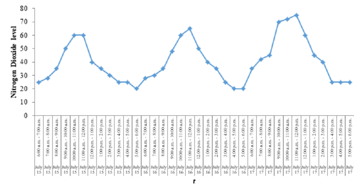
From the above time-series plot, it is clear that plot shows upward trend. Also, there exists seasonal pattern.
(b)
Find a multiple regression equation that represents seasonal effect using dummy variables for the given data.
(b)
Answer to Problem 25P
The regression equation is,
Explanation of Solution
Dummy variables are defined as given below:
Also, all the dummy variables are 0 when the reading time corresponds to 5:00 p.m. to 6:00 p.m.
The given data is entered as given below:
| Hourly Dummy Variables | |||||||||||||
| Date | Hour | yt | 1 | 2 | 3 | 4 | 5 | 6 | 7 | 8 | 9 | 10 | 11 |
| July 15 | 6:00 a.m. - 7:00 a.m. | 25 | 1 | 0 | 0 | 0 | 0 | 0 | 0 | 0 | 0 | 0 | 0 |
| July 15 | 7:00 a.m. - 8:00 a.m. | 28 | 0 | 1 | 0 | 0 | 0 | 0 | 0 | 0 | 0 | 0 | 0 |
| July 15 | 8:00 a.m. - 9:00 a.m. | 35 | 0 | 0 | 1 | 0 | 0 | 0 | 0 | 0 | 0 | 0 | 0 |
| July 15 | 9:00 a.m. - 10:00 a.m. | 50 | 0 | 0 | 0 | 1 | 0 | 0 | 0 | 0 | 0 | 0 | 0 |
| July 15 | 10:00 a.m. - 11:00 a.m. | 60 | 0 | 0 | 0 | 0 | 1 | 0 | 0 | 0 | 0 | 0 | 0 |
| July 15 | 11:00 a.m. - 12:00 p.m. | 60 | 0 | 0 | 0 | 0 | 0 | 1 | 0 | 0 | 0 | 0 | 0 |
| July 15 | 12:00 p.m. - 1:00 p.m. | 40 | 0 | 0 | 0 | 0 | 0 | 0 | 1 | 0 | 0 | 0 | 0 |
| July 15 | 1:00 p.m. - 2:00 p.m. | 35 | 0 | 0 | 0 | 0 | 0 | 0 | 0 | 1 | 0 | 0 | 0 |
| July 15 | 2:00 p.m. - 3:00 p.m. | 30 | 0 | 0 | 0 | 0 | 0 | 0 | 0 | 0 | 1 | 0 | 0 |
| July 15 | 3:00 p.m. - 4:00 p.m. | 25 | 0 | 0 | 0 | 0 | 0 | 0 | 0 | 0 | 0 | 1 | 0 |
| July 15 | 4:00 p.m. - 5:00 p.m. | 25 | 0 | 0 | 0 | 0 | 0 | 0 | 0 | 0 | 0 | 0 | 1 |
| July 15 | 5:00 p.m. - 6:00 p.m. | 20 | 0 | 0 | 0 | 0 | 0 | 0 | 0 | 0 | 0 | 0 | 0 |
| July 16 | 6:00 a.m. - 7:00 a.m. | 28 | 1 | 0 | 0 | 0 | 0 | 0 | 0 | 0 | 0 | 0 | 0 |
| July 16 | 7:00 a.m. - 8:00 a.m. | 30 | 0 | 1 | 0 | 0 | 0 | 0 | 0 | 0 | 0 | 0 | 0 |
| July 16 | 8:00 a.m. - 9:00 a.m. | 35 | 0 | 0 | 1 | 0 | 0 | 0 | 0 | 0 | 0 | 0 | 0 |
| July 16 | 9:00 a.m. - 10:00 a.m. | 48 | 0 | 0 | 0 | 1 | 0 | 0 | 0 | 0 | 0 | 0 | 0 |
| July 16 | 10:00 a.m. - 11:00 a.m. | 60 | 0 | 0 | 0 | 0 | 1 | 0 | 0 | 0 | 0 | 0 | 0 |
| July 16 | 11:00 a.m. - 12:00 p.m. | 65 | 0 | 0 | 0 | 0 | 0 | 1 | 0 | 0 | 0 | 0 | 0 |
| July 16 | 12:00 p.m. - 1:00 p.m. | 50 | 0 | 0 | 0 | 0 | 0 | 0 | 1 | 0 | 0 | 0 | 0 |
| July 16 | 1:00 p.m. - 2:00 p.m. | 40 | 0 | 0 | 0 | 0 | 0 | 0 | 0 | 1 | 0 | 0 | 0 |
| July 16 | 2:00 p.m. - 3:00 p.m. | 35 | 0 | 0 | 0 | 0 | 0 | 0 | 0 | 0 | 1 | 0 | 0 |
| July 16 | 3:00 p.m. - 4:00 p.m. | 25 | 0 | 0 | 0 | 0 | 0 | 0 | 0 | 0 | 0 | 1 | 0 |
| July 16 | 4:00 p.m. - 5:00 p.m. | 20 | 0 | 0 | 0 | 0 | 0 | 0 | 0 | 0 | 0 | 0 | 1 |
| July 16 | 5:00 p.m. - 6:00 p.m. | 20 | 0 | 0 | 0 | 0 | 0 | 0 | 0 | 0 | 0 | 0 | 0 |
| July 17 | 6:00 a.m. - 7:00 a.m. | 35 | 1 | 0 | 0 | 0 | 0 | 0 | 0 | 0 | 0 | 0 | 0 |
| July 17 | 7:00 a.m. - 8:00 a.m. | 42 | 0 | 1 | 0 | 0 | 0 | 0 | 0 | 0 | 0 | 0 | 0 |
| July 17 | 8:00 a.m. - 9:00 a.m. | 45 | 0 | 0 | 1 | 0 | 0 | 0 | 0 | 0 | 0 | 0 | 0 |
| July 17 | 9:00 a.m. - 10:00 a.m. | 70 | 0 | 0 | 0 | 1 | 0 | 0 | 0 | 0 | 0 | 0 | 0 |
| July 17 | 10:00 a.m. - 11:00 a.m. | 72 | 0 | 0 | 0 | 0 | 1 | 0 | 0 | 0 | 0 | 0 | 0 |
| July 17 | 11:00 a.m. - 12:00 p.m. | 75 | 0 | 0 | 0 | 0 | 0 | 1 | 0 | 0 | 0 | 0 | 0 |
| July 17 | 12:00 p.m. - 1:00 p.m. | 60 | 0 | 0 | 0 | 0 | 0 | 0 | 1 | 0 | 0 | 0 | 0 |
| July 17 | 1:00 p.m. - 2:00 p.m. | 45 | 0 | 0 | 0 | 0 | 0 | 0 | 0 | 1 | 0 | 0 | 0 |
| July 17 | 2:00 p.m. - 3:00 p.m. | 40 | 0 | 0 | 0 | 0 | 0 | 0 | 0 | 0 | 1 | 0 | 0 |
| July 17 | 3:00 p.m. - 4:00 p.m. | 25 | 0 | 0 | 0 | 0 | 0 | 0 | 0 | 0 | 0 | 1 | 0 |
| July 17 | 4:00 p.m. - 5:00 p.m. | 25 | 0 | 0 | 0 | 0 | 0 | 0 | 0 | 0 | 0 | 0 | 1 |
| July 17 | 5:00 p.m. - 6:00 p.m. | 25 | 0 | 0 | 0 | 0 | 0 | 0 | 0 | 0 | 0 | 0 | 0 |
Step-by-step procedure to obtain multiple linear regression line is given below.
- Enter the data in columns A to M.
- Click on Data tab and then Data Analysis.
- Select Regression and click ok.
- In Input Y
Range select, $B$2:$B$37 and Input X Range select $C$2:$M$37 - Click Ok.
The output is given below:
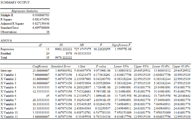
From the output the regression equation is,
Here, X Variable 1 represents Hour1, X Variable 2 represents Hour2, … X variable 11 represents Hour11.
(c)
Find the estimates of the levels of nitrogen for July 18 using the model developed in part (b).
(c)
Explanation of Solution
From part (b), the regression equation is,
Forecast for July 18 is obtained as given below:
| Hourly forecast | Calculation | |
| Hour1 | 29.34 | |
| Hour2 | 33.34 | |
| Hour3 | 38.34 | |
| Hour4 | 56 | |
| Hour5 | 64 | |
| Hour6 | 66.67 | |
| Hour7 | 50 | |
| Hour8 | 40 | |
| Hour9 | 35 | |
| Hour10 | 25 | |
| Hour11 | 23.34 | |
| Hour12 | 21.67 | 21.67 |
(d)
Construct a multiple regression equation that represents seasonal effect using dummy variables and a t variable for the given data.
(d)
Answer to Problem 25P
The regression equation is,
Explanation of Solution
Create a variable t such that t = 1 for hour 1 on July 15, t = 2 for hour 2 on July 2, …, t = 36 for hour 12 on July 18.
The given data is entered as given below:
| Hourly Dummy Variables | ||||||||||||||
| Date | Hour | yt | 1 | 2 | 3 | 4 | 5 | 6 | 7 | 8 | 9 | 10 | 11 | t |
| July 15 | 6:00 a.m. - 7:00 a.m. | 25 | 1 | 0 | 0 | 0 | 0 | 0 | 0 | 0 | 0 | 0 | 0 | 1 |
| July 15 | 7:00 a.m. - 8:00 a.m. | 28 | 0 | 1 | 0 | 0 | 0 | 0 | 0 | 0 | 0 | 0 | 0 | 2 |
| July 15 | 8:00 a.m. - 9:00 a.m. | 35 | 0 | 0 | 1 | 0 | 0 | 0 | 0 | 0 | 0 | 0 | 0 | 3 |
| July 15 | 9:00 a.m. - 10:00 a.m. | 50 | 0 | 0 | 0 | 1 | 0 | 0 | 0 | 0 | 0 | 0 | 0 | 4 |
| July 15 | 10:00 a.m. - 11:00 a.m. | 60 | 0 | 0 | 0 | 0 | 1 | 0 | 0 | 0 | 0 | 0 | 0 | 5 |
| July 15 | 11:00 a.m. - 12:00 p.m. | 60 | 0 | 0 | 0 | 0 | 0 | 1 | 0 | 0 | 0 | 0 | 0 | 6 |
| July 15 | 12:00 p.m. - 1:00 p.m. | 40 | 0 | 0 | 0 | 0 | 0 | 0 | 1 | 0 | 0 | 0 | 0 | 7 |
| July 15 | 1:00 p.m. - 2:00 p.m. | 35 | 0 | 0 | 0 | 0 | 0 | 0 | 0 | 1 | 0 | 0 | 0 | 8 |
| July 15 | 2:00 p.m. - 3:00 p.m. | 30 | 0 | 0 | 0 | 0 | 0 | 0 | 0 | 0 | 1 | 0 | 0 | 9 |
| July 15 | 3:00 p.m. - 4:00 p.m. | 25 | 0 | 0 | 0 | 0 | 0 | 0 | 0 | 0 | 0 | 1 | 0 | 10 |
| July 15 | 4:00 p.m. - 5:00 p.m. | 25 | 0 | 0 | 0 | 0 | 0 | 0 | 0 | 0 | 0 | 0 | 1 | 11 |
| July 15 | 5:00 p.m. - 6:00 p.m. | 20 | 0 | 0 | 0 | 0 | 0 | 0 | 0 | 0 | 0 | 0 | 0 | 12 |
| July 16 | 6:00 a.m. - 7:00 a.m. | 28 | 1 | 0 | 0 | 0 | 0 | 0 | 0 | 0 | 0 | 0 | 0 | 13 |
| July 16 | 7:00 a.m. - 8:00 a.m. | 30 | 0 | 1 | 0 | 0 | 0 | 0 | 0 | 0 | 0 | 0 | 0 | 14 |
| July 16 | 8:00 a.m. - 9:00 a.m. | 35 | 0 | 0 | 1 | 0 | 0 | 0 | 0 | 0 | 0 | 0 | 0 | 15 |
| July 16 | 9:00 a.m. - 10:00 a.m. | 48 | 0 | 0 | 0 | 1 | 0 | 0 | 0 | 0 | 0 | 0 | 0 | 16 |
| July 16 | 10:00 a.m. - 11:00 a.m. | 60 | 0 | 0 | 0 | 0 | 1 | 0 | 0 | 0 | 0 | 0 | 0 | 17 |
| July 16 | 11:00 a.m. - 12:00 p.m. | 65 | 0 | 0 | 0 | 0 | 0 | 1 | 0 | 0 | 0 | 0 | 0 | 18 |
| July 16 | 12:00 p.m. - 1:00 p.m. | 50 | 0 | 0 | 0 | 0 | 0 | 0 | 1 | 0 | 0 | 0 | 0 | 19 |
| July 16 | 1:00 p.m. - 2:00 p.m. | 40 | 0 | 0 | 0 | 0 | 0 | 0 | 0 | 1 | 0 | 0 | 0 | 20 |
| July 16 | 2:00 p.m. - 3:00 p.m. | 35 | 0 | 0 | 0 | 0 | 0 | 0 | 0 | 0 | 1 | 0 | 0 | 21 |
| July 16 | 3:00 p.m. - 4:00 p.m. | 25 | 0 | 0 | 0 | 0 | 0 | 0 | 0 | 0 | 0 | 1 | 0 | 22 |
| July 16 | 4:00 p.m. - 5:00 p.m. | 20 | 0 | 0 | 0 | 0 | 0 | 0 | 0 | 0 | 0 | 0 | 1 | 23 |
| July 16 | 5:00 p.m. - 6:00 p.m. | 20 | 0 | 0 | 0 | 0 | 0 | 0 | 0 | 0 | 0 | 0 | 0 | 24 |
| July 17 | 6:00 a.m. - 7:00 a.m. | 35 | 1 | 0 | 0 | 0 | 0 | 0 | 0 | 0 | 0 | 0 | 0 | 25 |
| July 17 | 7:00 a.m. - 8:00 a.m. | 42 | 0 | 1 | 0 | 0 | 0 | 0 | 0 | 0 | 0 | 0 | 0 | 26 |
| July 17 | 8:00 a.m. - 9:00 a.m. | 45 | 0 | 0 | 1 | 0 | 0 | 0 | 0 | 0 | 0 | 0 | 0 | 27 |
| July 17 | 9:00 a.m. - 10:00 a.m. | 70 | 0 | 0 | 0 | 1 | 0 | 0 | 0 | 0 | 0 | 0 | 0 | 28 |
| July 17 | 10:00 a.m. - 11:00 a.m. | 72 | 0 | 0 | 0 | 0 | 1 | 0 | 0 | 0 | 0 | 0 | 0 | 29 |
| July 17 | 11:00 a.m. - 12:00 p.m. | 75 | 0 | 0 | 0 | 0 | 0 | 1 | 0 | 0 | 0 | 0 | 0 | 30 |
| July 17 | 12:00 p.m. - 1:00 p.m. | 60 | 0 | 0 | 0 | 0 | 0 | 0 | 1 | 0 | 0 | 0 | 0 | 31 |
| July 17 | 1:00 p.m. - 2:00 p.m. | 45 | 0 | 0 | 0 | 0 | 0 | 0 | 0 | 1 | 0 | 0 | 0 | 32 |
| July 17 | 2:00 p.m. - 3:00 p.m. | 40 | 0 | 0 | 0 | 0 | 0 | 0 | 0 | 0 | 1 | 0 | 0 | 33 |
| July 17 | 3:00 p.m. - 4:00 p.m. | 25 | 0 | 0 | 0 | 0 | 0 | 0 | 0 | 0 | 0 | 1 | 0 | 34 |
| July 17 | 4:00 p.m. - 5:00 p.m. | 25 | 0 | 0 | 0 | 0 | 0 | 0 | 0 | 0 | 0 | 0 | 1 | 35 |
| July 17 | 5:00 p.m. - 6:00 p.m. | 25 | 0 | 0 | 0 | 0 | 0 | 0 | 0 | 0 | 0 | 0 | 0 | 36 |
Step-by-step procedure to obtain multiple linear regression line is given below.
- Enter the data in columns A to N.
- Click on Data tab and then Data Analysis.
- Select Regression and click ok.
- In Input Y Range select, $B$2:$B$37 and Input X Range select $C$2:$N$37
- Click Ok.
The output is given below:
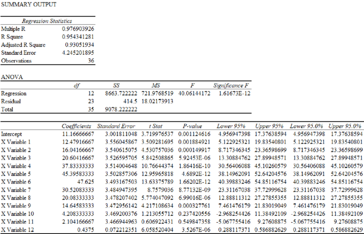
From the output the regression equation is,
Here, X Variable 1 represents Hour1, X Variable 2 represents Hour2,… X variable 11 represents Hour11 and X variable 12 represents t.
(e)
Calculate the estimates of the levels of nitrogen for July 18 using the model developed in part (d).
(e)
Explanation of Solution
From part (d), the regression equation is,
Forecast for July 18 is given below:
| Hourly forecast | T | Calculation | |
| 1 | 37 | 39.93 | |
| 2 | 38 | 43.93 | |
| 3 | 39 | 48.93 | |
| 4 | 40 | 66.6 | |
| 5 | 41 | 74.71 | |
| 6 | 42 | 77.28 | |
| 7 | 43 | 60.61 | |
| 8 | 44 | 50.61 | |
| 9 | 45 | 45.62 | |
| 10 | 46 | 35.62 | |
| 11 | 47 | 33.95 | |
| 12 | 48 | 32.29 |
(f)
Justify which of the models (b) or (d) is effective.
(f)
Answer to Problem 25P
Model (d) is preferred.
Explanation of Solution
For the multiple regression equation developed in part (b), MSE is obtained as given below:
| Date | Hour | yt | Forecast | Forecast Error | Squared Forecast Error |
| 15-Jul | 6:00 a.m. - 7:00 a.m. | 25 | 29.34 | -4.34 | 18.8356 |
| 15-Jul | 7:00 a.m. - 8:00 a.m. | 28 | 33.34 | -5.34 | 28.5156 |
| 15-Jul | 8:00 a.m. - 9:00 a.m. | 35 | 38.34 | -3.34 | 11.1556 |
| 15-Jul | 9:00 a.m. - 10:00 a.m. | 50 | 56 | -6 | 36 |
| 15-Jul | 10:00 a.m. - 11:00 a.m. | 60 | 64 | -4 | 16 |
| 15-Jul | 11:00 a.m. - 12:00 p.m. | 60 | 66.67 | -6.67 | 44.4889 |
| 15-Jul | 12:00 p.m. - 1:00 p.m. | 40 | 50 | -10 | 100 |
| 15-Jul | 1:00 p.m. - 2:00 p.m. | 35 | 40 | -5 | 25 |
| 15-Jul | 2:00 p.m. - 3:00 p.m. | 30 | 35 | -5 | 25 |
| 15-Jul | 3:00 p.m. - 4:00 p.m. | 25 | 25 | 0 | 0 |
| 15-Jul | 4:00 p.m. - 5:00 p.m. | 25 | 23.34 | 1.66 | 2.7556 |
| 15-Jul | 5:00 p.m. - 6:00 p.m. | 20 | 21.67 | -1.67 | 2.7889 |
| 16-Jul | 6:00 a.m. - 7:00 a.m. | 28 | 29.34 | -1.34 | 1.7956 |
| 16-Jul | 7:00 a.m. - 8:00 a.m. | 30 | 33.34 | -3.34 | 11.1556 |
| 16-Jul | 8:00 a.m. - 9:00 a.m. | 35 | 38.34 | -3.34 | 11.1556 |
| 16-Jul | 9:00 a.m. - 10:00 a.m. | 48 | 56 | -8 | 64 |
| 16-Jul | 10:00 a.m. - 11:00 a.m. | 60 | 64 | -4 | 16 |
| 16-Jul | 11:00 a.m. - 12:00 p.m. | 65 | 66.67 | -1.67 | 2.7889 |
| 16-Jul | 12:00 p.m. - 1:00 p.m. | 50 | 50 | 0 | 0 |
| 16-Jul | 1:00 p.m. - 2:00 p.m. | 40 | 40 | 0 | 0 |
| 16-Jul | 2:00 p.m. - 3:00 p.m. | 35 | 35 | 0 | 0 |
| 16-Jul | 3:00 p.m. - 4:00 p.m. | 25 | 25 | 0 | 0 |
| 16-Jul | 4:00 p.m. - 5:00 p.m. | 20 | 23.34 | -3.34 | 11.1556 |
| 16-Jul | 5:00 p.m. - 6:00 p.m. | 20 | 21.67 | -1.67 | 2.7889 |
| 17-Jul | 6:00 a.m. - 7:00 a.m. | 35 | 29.34 | 5.66 | 32.0356 |
| 17-Jul | 7:00 a.m. - 8:00 a.m. | 42 | 33.34 | 8.66 | 74.9956 |
| 17-Jul | 8:00 a.m. - 9:00 a.m. | 45 | 38.34 | 6.66 | 44.3556 |
| 17-Jul | 9:00 a.m. - 10:00 a.m. | 70 | 56 | 14 | 196 |
| 17-Jul | 10:00 a.m. - 11:00 a.m. | 72 | 64 | 8 | 64 |
| 17-Jul | 11:00 a.m. - 12:00 p.m. | 75 | 66.67 | 8.33 | 69.3889 |
| 17-Jul | 12:00 p.m. - 1:00 p.m. | 60 | 50 | 10 | 100 |
| 17-Jul | 1:00 p.m. - 2:00 p.m. | 45 | 40 | 5 | 25 |
| 17-Jul | 2:00 p.m. - 3:00 p.m. | 40 | 35 | 5 | 25 |
| 17-Jul | 3:00 p.m. - 4:00 p.m. | 25 | 25 | 0 | 0 |
| 17-Jul | 4:00 p.m. - 5:00 p.m. | 25 | 23.34 | 1.66 | 2.7556 |
| 17-Jul | 5:00 p.m. - 6:00 p.m. | 25 | 21.67 | 3.33 | 11.0889 |
| 1076.001 |
For the multiple regression equation developed in part (d), MSE is obtained as given below:
| Date | Hour | t | yt | Forecast | Forecast Error | Squared Forecast Error |
| 15-Jul | 6:00 a.m. - 7:00 a.m. | 1 | 25 | 24.09 | 0.91 | 0.8281 |
| 15-Jul | 7:00 a.m. - 8:00 a.m. | 2 | 28 | 28.09 | -0.09 | 0.0081 |
| 15-Jul | 8:00 a.m. - 9:00 a.m. | 3 | 35 | 33.09 | 1.91 | 3.6481 |
| 15-Jul | 9:00 a.m. - 10:00 a.m. | 4 | 50 | 50.76 | -0.76 | 0.5776 |
| 15-Jul | 10:00 a.m. - 11:00 a.m. | 5 | 60 | 58.87 | 1.13 | 1.2769 |
| 15-Jul | 11:00 a.m. - 12:00 p.m. | 6 | 60 | 61.44 | -1.44 | 2.0736 |
| 15-Jul | 12:00 p.m. - 1:00 p.m. | 7 | 40 | 44.77 | -4.77 | 22.7529 |
| 15-Jul | 1:00 p.m. - 2:00 p.m. | 8 | 35 | 34.77 | 0.23 | 0.0529 |
| 15-Jul | 2:00 p.m. - 3:00 p.m. | 9 | 30 | 29.78 | 0.22 | 0.0484 |
| 15-Jul | 3:00 p.m. - 4:00 p.m. | 10 | 25 | 19.78 | 5.22 | 27.2484 |
| 15-Jul | 4:00 p.m. - 5:00 p.m. | 11 | 25 | 18.11 | 6.89 | 47.4721 |
| 15-Jul | 5:00 p.m. - 6:00 p.m. | 12 | 20 | 16.45 | 3.55 | 12.6025 |
| 16-Jul | 6:00 a.m. - 7:00 a.m. | 13 | 28 | 29.37 | -1.37 | 1.8769 |
| 16-Jul | 7:00 a.m. - 8:00 a.m. | 14 | 30 | 33.37 | -3.37 | 11.3569 |
| 16-Jul | 8:00 a.m. - 9:00 a.m. | 15 | 35 | 38.37 | -3.37 | 11.3569 |
| 16-Jul | 9:00 a.m. - 10:00 a.m. | 16 | 48 | 56.04 | -8.04 | 64.6416 |
| 16-Jul | 10:00 a.m. - 11:00 a.m. | 17 | 60 | 64.15 | -4.15 | 17.2225 |
| 16-Jul | 11:00 a.m. - 12:00 p.m. | 18 | 65 | 66.72 | -1.72 | 2.9584 |
| 16-Jul | 12:00 p.m. - 1:00 p.m. | 19 | 50 | 50.05 | -0.05 | 0.0025 |
| 16-Jul | 1:00 p.m. - 2:00 p.m. | 20 | 40 | 40.05 | -0.05 | 0.0025 |
| 16-Jul | 2:00 p.m. - 3:00 p.m. | 21 | 35 | 35.06 | -0.06 | 0.0036 |
| 16-Jul | 3:00 p.m. - 4:00 p.m. | 22 | 25 | 25.06 | -0.06 | 0.0036 |
| 16-Jul | 4:00 p.m. - 5:00 p.m. | 23 | 20 | 23.39 | -3.39 | 11.4921 |
| 16-Jul | 5:00 p.m. - 6:00 p.m. | 24 | 20 | 21.73 | -1.73 | 2.9929 |
| 17-Jul | 6:00 a.m. - 7:00 a.m. | 25 | 35 | 34.65 | 0.35 | 0.1225 |
| 17-Jul | 7:00 a.m. - 8:00 a.m. | 26 | 42 | 38.65 | 3.35 | 11.2225 |
| 17-Jul | 8:00 a.m. - 9:00 a.m. | 27 | 45 | 43.65 | 1.35 | 1.8225 |
| 17-Jul | 9:00 a.m. - 10:00 a.m. | 28 | 70 | 61.32 | 8.68 | 75.3424 |
| 17-Jul | 10:00 a.m. - 11:00 a.m. | 29 | 72 | 69.43 | 2.57 | 6.6049 |
| 17-Jul | 11:00 a.m. - 12:00 p.m. | 30 | 75 | 72 | 3 | 9 |
| 17-Jul | 12:00 p.m. - 1:00 p.m. | 31 | 60 | 55.33 | 4.67 | 21.8089 |
| 17-Jul | 1:00 p.m. - 2:00 p.m. | 32 | 45 | 45.33 | -0.33 | 0.1089 |
| 17-Jul | 2:00 p.m. - 3:00 p.m. | 33 | 40 | 40.34 | -0.34 | 0.1156 |
| 17-Jul | 3:00 p.m. - 4:00 p.m. | 34 | 25 | 30.34 | -5.34 | 28.5156 |
| 17-Jul | 4:00 p.m. - 5:00 p.m. | 35 | 25 | 28.67 | -3.67 | 13.4689 |
| 17-Jul | 5:00 p.m. - 6:00 p.m. | 36 | 25 | 27.01 | -2.01 | 4.0401 |
| 414.6728 |
MSE for model in (d) is smaller than MSE for the model in (b). Thus, model (d) is preferred.
Want to see more full solutions like this?
Chapter 5 Solutions
Essentials Of Business Analytics


- Now consider a bag of ten colorful marbles. You reach into the bag 100 times. Each time you pull out a marble, write down what color it was, then put it back in the bag and do it again. You record the following data: Table describing marble frequency Color Frequency Red 22 Yellow 9 Green 41 Blue 28arrow_forwardFor the first two weeks of the month of January 2022, the daily average of calls for roadside assistance from motorcycle drivers was kept track of. These were the outcomes: Find the Mode: Construct a frequency graph:arrow_forwardThe median home value in Mississippi and Maryland (adjusted for inflation) are shown below: If we assume that the house values are changing linearly,a) In which state have home values increased at a higher rate? b) If these trends were to continue, what would be the median home value in Mississippi in 2010?$arrow_forward
- MORTALITY RATE Table 3.5 provides the number of deaths from all causes and from accidents (unintentional injuries) by age group in the United States in 2002. Review the following rates. Determine what to call each one, then calculate it using the data provided in Table. 1. Unintentional-injury-specific mortality rate for the entire population. Calculate cause-specific mortality rate. 2. All-cause mortality rate for 25-34 years old. Calculate the age-specific mortality rate. 3. All-cause mortality among males. Calculate the sex-specific mortality rate. 4. Unintentional-injury specific mortality among 25 to 34 years old males. Calculate the is a cause-specific, age-specific, and sex-specific mortality rate Table 3.5 All-Cause and Unintentional Injury Mortality and Estimated Population by Age Group, For Both Sexes and For Males Alone- United States, 2002 All Races, Both Sexes All Races, Males Age group (years) All Causes Unintentional Estimated All Unintentional Estimated Injuries Pop. (x…arrow_forwarders each of its retail employees activates we of activations and satisfactic Activations Satisfaction O 37 8.0 22 7.9 37 8.5 37 9.0 18 6.1 27 7.0 32 8.2 28 77 Print Done ade by an employee with a job-satisfaction score of Doorsonarrow_forwardDuring one shift, the express lane clerk recorded how many times customers violated the "10 items or less" rule for his lane. In particular, he recorded how many items over the limit each violator placed on the conveyor belt. This data is summarized in the histogram below. NOTE: The last class actually represents "7 or more items," not just 7 items. Frequency 12+ 298 ans = 10- a 2 0.5 1.5 2.5 3.5 4.5 5.5 6.5 7.5 # items over 10 What is the frequency of times the limit was exceeded by at least 3 items?arrow_forward
- A restaurant uses comment cards to get feedback from its customers about newly added items to the menu. It recently introduced homemade organic veggie burgers. Customers who tried the new burger were asked if they would order it again. The data is summarized in the table and bar graph. A. Convert this table into a relative frequency Round answers to the nearest tenth. B. Based upon the bar chart and the relative frequency table, would you recommend that the restaurant owner keeps the organic veggie burger on the menu? Explain yourarrow_forwardIn 2019 a major appliance factory can produce 600 ovens daily . To make sure the temperature controls are calibrated properly, an oven is set to 350 degrees Fahrenheit . Once the display shows 350 is reached , the temperature of the oven is tested and recorded. A factory worker selects 50 ovens to test throughout the day. The recorded temperatures are evaluated (Please use the drop down menus to answer each question.) a. In this scenario, what value represents the population under study? 2019, 50,350, 600, or temperature b. In this scenario, what value represents the sample used for the study? 2019, 50,350, 600, or temperature c. What data type is the worker gathering ? 2019, 50,350, 600, or temperature d. What level of measurement does this type of data have? 2019, 50,350, 600, or temperaturearrow_forwardEach day, the office staff at Oasis Quick Shop prepares a frequency distribution and an ogive of sales transactions by dollar value of the transactions. Saturday's cumulative frequency ogive follows. The percentage of sales transactions on Saturday that were at least $100 each was a. 100 b. 10 c. 80 d. 20 e. 15arrow_forward
- The scores that golfers shot on 18 holes at a local course were tabulated. The results are shown in the following frequency distribution.arrow_forwardUse the table below to answer questions 1-3. Suppose we want to estimate the annual high temperatures of the hottest major cities in the United States. Below is data from 12 cities with the average annual temperature taken from 1971 to 2000 (https://www.statista.com/statistics/226809/us-cities-with-the-highest-annual-temperatures/). City Temperature (Fahrenheit) Phoenix, Arizona 87.2 Miami, Florida 84.3 Orlando, Florida 82.8 Riverside, California 80.9 Austin, Texas 79.8 Houston, Texas 79.7 San Antonio, Texas 80.3 Las Vegas, Nevada 80.1 Jacksonville, Florida 79.3 New Orleans, Louisiana 78.2 Tampa, Florida 81.7 Los Angeles, California 75.2 Flag question: Question 1 Question 1 State the population for this study. The population is____________ Question 2 State the sample for this study. The sample is_______________ Question 3 What are the variables for the study and classify each as…arrow_forwardA car dealership keeps track of how much it spends on advertising each month and of its monthly revenue. From this information, the list of advertising expenditures and probable associated revenues are shown in the table below.arrow_forward
 Big Ideas Math A Bridge To Success Algebra 1: Stu...AlgebraISBN:9781680331141Author:HOUGHTON MIFFLIN HARCOURTPublisher:Houghton Mifflin Harcourt
 Trigonometry (MindTap Course List)TrigonometryISBN:9781305652224Author:Charles P. McKeague, Mark D. TurnerPublisher:Cengage Learning
 Glencoe Algebra 1, Student Edition, 9780079039897...AlgebraISBN:9780079039897Author:CarterPublisher:McGraw Hill
 Holt Mcdougal Larson Pre-algebra: Student Edition...AlgebraISBN:9780547587776Author:HOLT MCDOUGALPublisher:HOLT MCDOUGAL
 Algebra: Structure And Method, Book 1AlgebraISBN:9780395977224Author:Richard G. Brown, Mary P. Dolciani, Robert H. Sorgenfrey, William L. ColePublisher:McDougal Littell