
Sub part (a):
Consumption schedule and marginal propensity to consume.
Sub part (a):
Explanation of Solution
Table -1 shows the consumption schedule:
Table -1
| Consumption | |
| 100 | 120 |
| 200 | 200 |
| 300 | 280 |
| 400 | 360 |
| 500 | 440 |
| 600 | 520 |
| 700 | 600 |
Figure 1 illustrates the level of consumption at different level of gross domestic product (GDP).
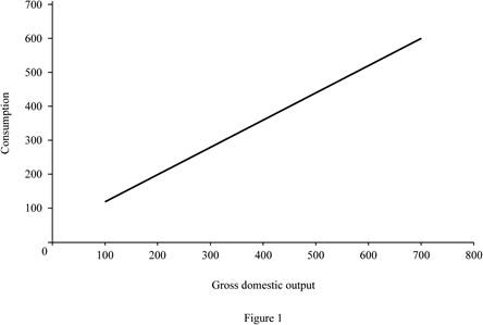
In Figure 1, the horizontal axis measures the gross domestic output and the vertical axis measures the consumption level.
Size of marginal propensity to consume (MPC) can be calculated as follows.
The size of marginal propensity to consume is 0.8.
Concept introduction:
Consumption schedule: Consumption schedule refers to the quantity of consumption at different levels of income.
Marginal propensity to consume (MPS): Marginal propensity to consume refers to the sensitivity of change in the consumption level due to the changes occurred in the income level.
Sub part (b):
Disposable income, tax rate, consumption schedule, marginal propensity to consume and multiplier.
Sub part (b):
Explanation of Solution
Disposable income (DI) can be calculated by using the following formula.
Substitute the respective values in Equation (1) to calculate the disposable income at the level of GDP $100.
Disposable income at the level of GDP $100 is $90.
Tax rate can be calculated by using the following formula.
Substitute the respective values in Equation (2) to calculate the tax rate at the level of GDP $100.
Tax rate at the level of GDP is 10%.
New consumption level can be calculated by using the following formula.
Substitute the respective values in Equation (3) to calculate the disposable income at the level of GDP $100. Since, the tax payment is equal amount of decrease in consumption for all the levels of GDP. The decreasing consumption for increasing $10 is assumed to be $8.
New consumption is $112.
Table -2 shows the values of disposable income, new consumption level after tax and the tax rate that are obtained by using Equations (1), (2) and (3).
Table -2
| Gross domestic product | Tax | DI | New consumption | Tax rate |
| 100 | 10 | 90 | 112 | 10% |
| 200 | 10 | 190 | 192 | 5% |
| 300 | 10 | 290 | 272 | 3.33% |
| 400 | 10 | 390 | 352 | 2.5% |
| 500 | 10 | 490 | 432 | 2% |
| 600 | 10 | 590 | 512 | 1.67% |
| 700 | 10 | 690 | 592 | 1.43% |
Size of marginal propensity to consume (MPC) can be calculated as follows.
The size of marginal propensity to consume is 0.8.
Multiplier: Multiplier refers to the ratio of change in the real GDP to the change in initial consumption, at a constant price rate. Multiplier is positively related to the marginal propensity to consumer and negatively related with the marginal propensity to save. Multiplier can be evaluated using the following formula:
Since the value of MPC remains the same for part (a) and part (b), there is no change in the value of multiplier. The value of multiplier is 5
Figure -2 illustrates the level of consumption at different level of gross domestic product (GDP) for lump sum tax (Regressive tax).
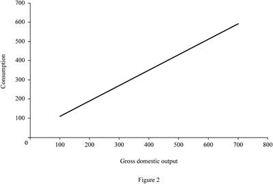
In Figure -2, the horizontal axis measures the gross domestic output and the vertical axis measures the consumption level.
Concept introduction:
Consumption schedule: Consumption schedule refers to the quantity of consumption at different levels of income.
Marginal propensity to consume (MPS): Marginal propensity to consume refers to the sensitivity of change in the consumption level due to the changes occurred in the income level.
Multiplier: Multiplier refers to the ratio of change in the real GDP to the change in initial consumption at constant price rate. Multiplier is positively related to the marginal propensity to consumer and negatively related with the marginal propensity to save.
Sub part (c):
Tax amount, consumption schedule, marginal propensity to consume and multiplier.
Sub part (c):
Explanation of Solution
Tax amount can be calculated by using the following formula.
Substitute the respective values in Equation (4) to calculate the tax amount at $100 GDP.
Tax amount is $10.
Table -3 shows the values of disposable income, new consumption level after tax and the tax rate that are obtained by using Equations (1), (2), (3) and (4). The change in tax amount is differing for different levels of GDP. The decreasing consumption for increasing each $10 is assumed to be $8 (Thus, if the tax payment is $30, then the consumption decreases by $24
Table -3
| Gross domestic product | Tax | DI | New consumption | Tax rate |
| 100 | 10 | 90 | 112 | 10% |
| 200 | 20 | 180 | 184 | 10% |
| 300 | 30 | 270 | 256 | 10% |
| 400 | 40 | 360 | 328 | 10% |
| 500 | 50 | 450 | 400 | 10% |
| 600 | 60 | 540 | 472 | 10% |
| 700 | 70 | 630 | 544 | 10% |
Multiplier: Multiplier refers to the ratio of change in the real GDP to the change in initial consumption, at a constant price rate. Multiplier is positively related to the marginal propensity to consumer and negatively related with the marginal propensity to save. Multiplier can be evaluated using the following formula:
Since the value of MPC different for part (a) and part (c), the value of multiplier for both the part is different. The value of multiplier is 3.57
Figure -3 illustrates the level of consumption at different level of gross domestic product (GDP) for proportional tax.
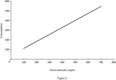
In Figure -3, the horizontal axis measures the gross domestic output and the vertical axis measures the consumption level.
Concept introduction:
Consumption schedule: Consumption schedule refers to the quantity of consumption at different levels of income.
Marginal propensity to consume (MPS): Marginal propensity to consume refers to the sensitivity of change in the consumption level due to the changes occurred in the income level.
Multiplier: Multiplier refers to the ratio of change in the real GDP to the change in initial consumption at constant price rate. Multiplier is positively related to the marginal propensity to consumer and negatively related with the marginal propensity to save.
Sub part (d):
consumption schedule, marginal propensity to consume and multiplier.
Sub part (d):
Explanation of Solution
Marginal propensity to consume can be calculated by using the following formula.
Substitute the respective values in Equation (5) to calculate the MPC at $100 GDP.
The value of MPC is 0.72.
Table -4 shows the values of disposable income, new consumption level after tax and the tax rate that are obtained by using Equations (1), (2), (3), (4) and (5). The change in tax amount is differing for different levels of GDP. The decreasing consumption for increasing each $10 is assumed to be $8 (Thus, if the tax payment is $20, then the consumption decreases by $16
Table -3
| Gross domestic product | Tax | DI | New consumption | Tax rate | MPC |
| 100 | 0 | 100 | 120 | 0% | |
| 200 | 10 | 190 | 192 | 5% | 0.8 |
| 300 | 30 | 270 | 256 | 10% | 0.64 |
| 400 | 60 | 340 | 312 | 15% | 0.56 |
| 500 | 100 | 400 | 360 | 20% | 0.48 |
| 600 | 150 | 450 | 400 | 25% | 0.4 |
| 700 | 210 | 490 | 432 | 30% | 0.32 |
Multiplier: Multiplier refers to the ratio of change in the real GDP to the change in initial consumption, at a constant price rate. Multiplier is positively related to the marginal propensity to consumer and negatively related with the marginal propensity to save.
Multiplier value is differing for each level of GDP. When the tax rate increases, it reduces the value of MPC. Since the value of MPC decreases, the value of multiplier will also decrease.
Figure 4 illustrates the level of consumption at different level of gross domestic product (GDP) for progressive tax.
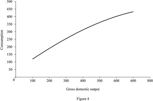
In Figure 4, the horizontal axis measures the gross domestic output and the vertical axis measures the consumption level.
Concept introduction:
Consumption schedule: Consumption schedule refers to the quantity of consumption at different levels of income.
Marginal propensity to consume (MPS): Marginal propensity to consume refers to the sensitivity of change in the consumption level due to the changes occurred in the income level.
Multiplier: Multiplier refers to the ratio of change in the real GDP to the change in initial consumption at constant price rate. Multiplier is positively related to the marginal propensity to consumer and negatively related with the marginal propensity to save.
Sup part (e):
Marginal propensity to consume and multiplier.
Sup part (e):
Explanation of Solution
Figure 1, Figure 2, Figure 3 and Figure 4 reveals that the proportional and progressive tax system reduces the value of MPC, so that the value of multiplier also decreases. The regressive tax system (Lump sum tax) does not alter the MPC. Since there is no change in the MPC, the multiplier remains the same.
Concept introduction:
Marginal propensity to consume (MPS): Marginal propensity to consume refers to the sensitivity of change in the consumption level due to the changes occurred in the income level.
Progressive tax: Progressive tax refers to the higher income people paying higher tax amount than the lower income people.
Proportional tax: Proportional tax rate refers to the fixed tax rate regardless of income and the tax rate and is the same for all levels of income.
Regressive tax: Regressive tax refers to the higher income people paying lower percentage of tax amount and lower income people paying higher percentage of tax amount.
Multiplier: Multiplier refers to the ratio of change in the real GDP to the change in initial consumption at constant price rate. Multiplier is positively related to the marginal propensity to consumer and negatively related with the marginal propensity to save.
Want to see more full solutions like this?
Chapter 33 Solutions
Economics (Irwin Economics)

- Which of the following is correct? 1) Expansionary fiscal policy during a recession means cutting taxes, increasing government spending, or taking both actions. 2) The goal of expansionary fiscal policy is to rein in inflation. 3) Expansionary fiscal policy tends to lead to a smaller budget deficit. O 4) Expansionary fiscal policy is always better than contractionary fiscal policy for 4) the economy.arrow_forward9. Refer to the accompanying table in answering the questions that follow: L011.8 (1) Possible Levels (3) Aggregate Expenditures (2) Real Domestic (C, + 1, + X, + G), Millions of Employment, Output, Millions Millions 90 $500 $520 100 550 560 110 600 600 120 650 640 130 700 680 a. If full employment in this economy is 130 million, will there be an inflationary expenditure gap or a recessionary expenditure gap? What will be the consequence of this gap? By how much would aggregate expenditures in column 3 have to change at each level of GDP to eliminate the inflationary expenditure gap or the recessionary expenditure gap? What is the multiplier in this example? b. Will there be an inflationary expenditure gap or a recessionary expenditure gap if the full-employment level of output is $500 billion? By how much would aggregate expenditures in column 3 have to change at each level of GDP to eliminate the gap? What is the multiplier in this example? c. Assuming that investment, net exports,…arrow_forward2. L Give Up! Suppose the Japanese economy has been experiencing slow growth. As a result, the Prime Minister, who thinks John Maynard Keynes was the greatest economist ever, has decided to increase government spending. The Prime Minister asks the head of the economic council to determine the increase in government spending necessary to bring the economy to full employment. Assume there is a GDP gap of 1 trillion yen and the marginal propensity to consume (MPC) is 0.60. What advice should the head of the economic council give the Prime Minister? O The recessionary gap is equal to 400 billion yen. O The inflationary gap is equal to 400 billion yen. O The recessionary gap is equal to 625 billion yen. O The inflationary gap is equal to 625 billion yen.arrow_forward
- 5. Refer to the data in the table that accompanies problem 2. Suppose that the present equilibrium price level and level of real GDP are 100 and $225, and that data set B represents the relevant aggregate supply schedule for the economy. LO12.6 a. What must be the current amount of real output demanded at the 100 price level? b. If the amount of output demanded declined by $25 at the 100 price level shown in B, what would be the new equilibrium real GDP? In business суcle economists call this change in real terminology, what would GDP?arrow_forwardQUESTION 14 Assuming that the "equilibrium income" is $4,000 and the "full-employment" income is $8,000, which means a recessionary gap of $4,000, how much tax cut is needed to fill the gap if MPC is 0.50? O $7,000 O $5,000 O $3,000 O $4,000arrow_forwardReal GDP Consumption (dollars) expenditure (dollars) 10 22.5 20 30 30 37.5 40 45 50 52.5 60 60 2 LAS 160 * SAS 150 140 130 120 AD 4 8 12 16 20 24 Real GDP (trillions of 2000 dollars) In the above table and figure, supposed that there is no import or proportional tax. To pull the economy back to the long-run equilibrium, the government can conduct a balanced budget operation by spending $ trillion. O 1) 1 O 2) 2 O 3) 4 4) 8 el (GDP deflator, 2000 = 100) Coarrow_forward
- QUESTION 16 If the marginal propensity to save is 0.1, the marginal propensity to import is 0.1 and the marginal tax rate is 0.2, how much would consumption increase if income rises by £8billion? O a. 4.8 O b. 13.3 O c. 3.2 O d. 20 4arrow_forward4 Suppose that Alberta imposes a sales tax of 10 percent on all goods and services. An Albertan named Ralph then goes into a home improvement store in the provincial capital of Edmonton and buys a leaf blower that is priced at $200. With the 10 percent sales tax, his total comes to $220. How much of the $220 paid by Ralph will be counted in the national income and product accounts as private income (employee compensation, rents, interest, proprietors' income, and corporate profits) v (Click to select) $220 $200 $180 None of the abovearrow_forwardQUESTION 10 Assuming that the "equilibrium income" is $4,000 and the "full-employment" income is $8,000, which means a recessionary gap of $4,000, how much change in government expenditures is needed to fill the gap if MPC is 0.50? O $3,000 O $4,000 O $1,000 O $2,000arrow_forward
- Suppose that the investment demand curve in a certain economy is such that investment declines by $110 billion for every 1 percentage point increase in the real interest rate. Also, suppose that the investment demand curve shifts rightward by $190 billion at each real interest rate for every 1 percentage point increase in the expected rate of return from investment. If stimulus spending (an expansionary fiscal policy) by government increases the real interest rate by 2 percentage points, but also raises the expected rate of return on investment by 1 percentage point, how much investment, if any, will be crowded out? Instructions: Enter your answer as a whole number. billion %24arrow_forwardSuppose that the investment demand curve in a certain economy is such that investment declines by $110 billion for every 1 percentage point increase in the real interest rate. Also, suppose that the investment demand curve shifts rightward by $170 billion at each real interest rate for every 1 percentage point increase in the expected rate of return from investment. If stimulus spending (an expansionary fiscal policy) by government increases the real interest rate by 2 percentage points, but also raises the expected rate of return on investment by 1 percentage point, how much investment, if any, will be crowded out? Note:- Do not provide handwritten solution. Maintain accuracy and quality in your answer. Take care of plagiarism. Answer completely. You will get up vote for sure.arrow_forward4. Below is a list of domestic output and national income figures for a certain year. All figures are in billions. The questions that follow ask you to determine the major national income measures by both the expenditures and income approaches. The results you obtain with the different methods should be the same. LO7.4 Personal consumption expenditures $245 7. Net foreign factor income 4 Transfer payments 12 Rents 14 Consumption of fixed capital (depreciation) 27 Statistical discrepancy 8. Social Security contributions 20 Interest 13 Proprietors' income 33 Net exports 11 Dividends 16 Compensation of employees 223 Taxes on production and imports 18 Undistributed corporate profits 21 Personal taxes 26 19 Corporate income taxes 56 Corporate profits 72 Government purchases 33 Net private domestic investment 20 Personal saving a. Using the above data, determine GDP by both the expenditures approach and the income approach. Then determine NDP. b. Now determine NI in two ways: first, by…arrow_forward

 Principles of Economics (12th Edition)EconomicsISBN:9780134078779Author:Karl E. Case, Ray C. Fair, Sharon E. OsterPublisher:PEARSON
 Engineering Economy (17th Edition)EconomicsISBN:9780134870069Author:William G. Sullivan, Elin M. Wicks, C. Patrick KoellingPublisher:PEARSON
 Principles of Economics (MindTap Course List)EconomicsISBN:9781305585126Author:N. Gregory MankiwPublisher:Cengage Learning
 Managerial Economics: A Problem Solving ApproachEconomicsISBN:9781337106665Author:Luke M. Froeb, Brian T. McCann, Michael R. Ward, Mike ShorPublisher:Cengage Learning
 Managerial Economics & Business Strategy (Mcgraw-...EconomicsISBN:9781259290619Author:Michael Baye, Jeff PrincePublisher:McGraw-Hill Education