Videos
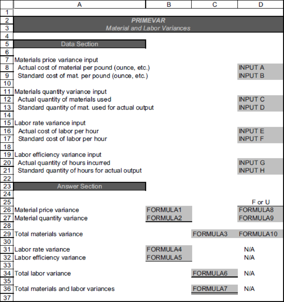
Close the PRIMEVAR4 file and open PRIMEVAR3. Click the Chart sheet tab. On the screen is a graphical representation of the variances computed in requirement 3. Review the chart and answer the following questions:
- a. Which variances does each bar represent?
A __________
B __________
C __________
D __________
- b. Which of the variances shown would be of most concern to management for immediate attention? (Consider groups of variances and materiality also.) Explain.
When the assignment is complete, close the file without saving it again.
Worksheet. McGrade Industries also has the following information regarding overhead for October: actual overhead $375,000, standard variable overhead of $3 per direct labor hour, and standard fixed overhead of $5 per direct labor hour (based on 47,000 hours budgeted). Modify the PRIMEVAR3 worksheet to compute all appropriate overhead variances. Preview the printout to make sure that the worksheet will print neatly on one page, and then print the worksheet. Save the completed file as PRIMEVART.
Hint: Insert several new rows in the Data Section and in the Answer Section.
Chart. Using the PRIMEVAR3 file, prepare a 3-D stacked bar chart to compare total
Want to see the full answer?
Check out a sample textbook solution
Chapter 24 Solutions
Excel Applications for Accounting Principles


- Please include excel formula Using the following returns, calculate the arithmetic average returns, the variances, and the standard deviations for X and Y. Input area: Year X Y 1 13% 27% 2 26% 36% 3 7% 11% 4 -5% -29% 5 11% 16% (Use cells A6 to C11 from the given information to complete this question. You must use the built-in Excel function to answers this question. Make sure to use the “sample” Excel formulas.) Output area: Asset X: Average return Variance Standard deviation Asset Y: Average return Variance Standard deviationarrow_forwardDownload the Applying Excel form and enter formulas in all cells that contain question marks. For example, in cell B30 enter the formula "= B20". Notes: In the text, variances are always displayed as positive numbers. To accomplish this, you can use the ABS() function in Excel. For example, the formula in cell C31 would be "=ABS(E31-B31)". Cells D31 through D39 and G31 through G39 already contain formulas to compute and display whether variances are Favorable or Unfavorable. Do not enter data or formulas into those cells-if you do, you will overwrite these formulas. After entering formulas in all of the cells that contained question marks, verify that the amounts match the numbers in the example in the text. Required: 1. Check your worksheet by changing the revenue in cell D4 to $16.00; the cost of ingredients in cell D5 to $6.50; and the wages and salaries in cell B6 to $10,000. The activity variance for net operating income should now be $850 U and the spending variance for total…arrow_forwardConsider the following time series: Construct a time series plot. What type of pattern exists in the data? Use simple linear regression analysis to find the parameters for the line that minimizes MSE for this time series. What is the forecast for t = 8?arrow_forward
- Can you show how to calculate the variance step by step without using excelarrow_forwardFind out coefficient of Variation (CV). Note: Use MS-EXCEL for the Calculation, Take Snapshot after analysisarrow_forwardPerformance Eval Variances: Refer to the pictures. One has the information and the second has the template. Thank you!arrow_forward
- Expected return and standard deviation. Use the following information to answer the questions: a. What is the expected return of each asset? b. What is the variance of each asset? c. What is the standard deviation of each asset? Hint: Make sure to round all intermediate calculations to at least seven (7) decimal places. The input instructions, phra answers you will type. Data table (Click on the following icon in order to copy its contents into a spreadsheet.) Return on Asset A in State of Economy Boom Normal Recession Probability of State 0.35 0.51 0.14 Print State 0.05 0.05 0.05 Done Return on Asset B in State 0.23 0.08 -0.05 Return on Asset C in State 0.33 0.17 -0.22arrow_forwardA1 fr Chapter 10: Applying Excel A В D E F 1 Chapter 10: Applying Excel 3 Data 4 Exhibit 10-1: Standard Cost Card Standard Quantity 2.9 pounds 5 Inputs Standard Price 6 Direct materials 7 Direct labor 8 Variable manufacturing overhead $4.00 per pound $22.00 per hour $6.00 per hour 0.60 hours 0.60 hours 9. 10 Actual results: Actual output Actual variable manufacturing overhead cost 13 2,000 units $7,140 Actual Quantity 6,500 pounds 11 12 Actual price $3.80 per pound $21.60 per hour 14 Actual direct materials cost 15 Actual direct labor cost 1,050 hours 16 17 Enter a formula into each of the cells marked with a ? below 18 Main Example: Chapter 10 19 20 Exhibit 10-4: Standard Cost Variance Analysis- Direct Materials 21 Standard Quantity Allowed for the Actual Output, at Standard Price 22 Actual Quantity of Input, at Standard Price 23 Actual Quantity of Input, at Actual Price 24 Direct materials variances: ? pounds x ? pounds x ? pounds x ? per pound = ? per pound = ? per pound = 25…arrow_forwardDefine the following terms, using graphs or equations to illustrate youranswers wherever feasible: d. Characteristic line; beta coefficient, barrow_forward
- Determine the variances for A, B, and C.arrow_forwardThe regression line in a scatterplot is also known as a(n): A. R-squared line. B. high-low line. C. outcome variable. D. linear trendline.arrow_forwardIn general, variance analysis is said to provide information about _________ and __________ variances.arrow_forward
 Excel Applications for Accounting PrinciplesAccountingISBN:9781111581565Author:Gaylord N. SmithPublisher:Cengage Learning
 Essentials of Business Analytics (MindTap Course ...StatisticsISBN:9781305627734Author:Jeffrey D. Camm, James J. Cochran, Michael J. Fry, Jeffrey W. Ohlmann, David R. AndersonPublisher:Cengage Learning