
Concept explainers
Videos
(a)
Section 1:
To graph: A scatterplot that shows the increase in GPA over time by hand and check whether the linear increase seems reasonable.
(a)
Section 1:
Explanation of Solution
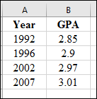
Graph: Plot the data from the provided table with GPA on y-axis and Year on x-axis.
Hence, the obtained graph is shown below:
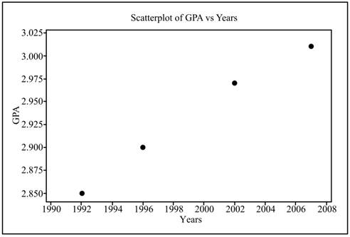
Interpretation: From the scatterplot, it can be seen that there is a linear dependency between GPA and year, which infers that the linear increase appears reasonable.
Section 2:
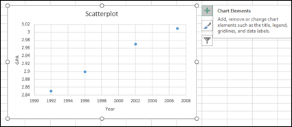
To graph: A scatterplot that shows the increase in GPA over time by using software and check whether the linear increase seems reasonable.
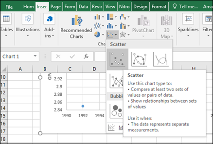
Section 2:
Explanation of Solution
Graph: Construct a scatterplot using excel as follows:
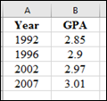
Step 1: Enter the data in Excel.
Step 2: Select the data. Click on Insert

Hence, the obtained graph is shown below:
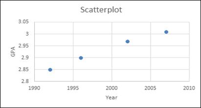
Interpretation: From the scatterplot, it can be seen that there is a linear dependency between GPA and year, so it can be said that by using software the results are same.
(b)
Section 1:
To find: The least square regression line for predicting GPA from year by hand.
(b)
Section 1:
Answer to Problem 30E
Solution: The regression line is
Explanation of Solution
Calculation: Compute the value of
Now, compute
Year (x) |
GPA (y) |
xy |
x2 |
1992 |
2.85 |
5677.2 |
3968064 |
1996 |
2.90 |
5788.4 |
3984016 |
2002 |
2.97 |
5945.9 |
4008004 |
2007 |
3.01 |
6041.1 |
4028049 |
Now, compute the value of
Compute the value of
Now, compute the value of
Hence, the obtained regression equation is
Interpretation: Therefore, it can be concluded from the obtained regression equation that the GPA increases by 0.011 times with the increase in year.
Section 2:
To graph: A scatterplot that shows the fitting of least-squares regression line by hand.
Section 2:
Explanation of Solution
Calculation: Obtain points for plotting on the graph using the regression equation as follows:
Let
Let
Let
Let
Now, plot these points of GPA on
Graph:
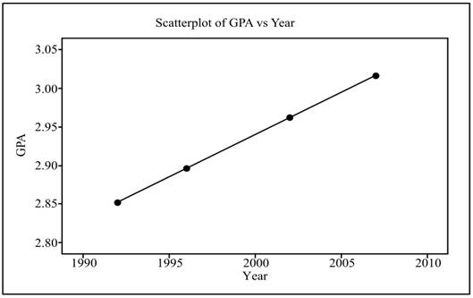
Interpretation: Therefore, it can be said that all the points lie on the regression line, so it can be concluded that the line is a good fit.
Section 3:
To find: The least square regression line for predicting GPA from year by software.
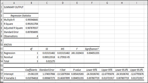
Section 3:
Answer to Problem 30E
Solution: The regression line is:
Explanation of Solution
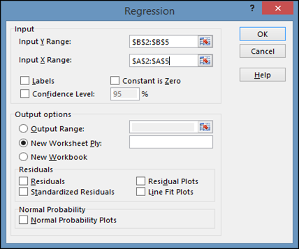
Calculation: Obtain the regression line using Excel as follows:
Step 1: Click on Data
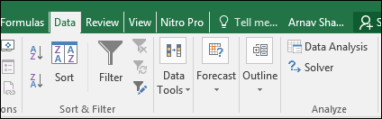
Step 3: Enter Y variable and X variable input
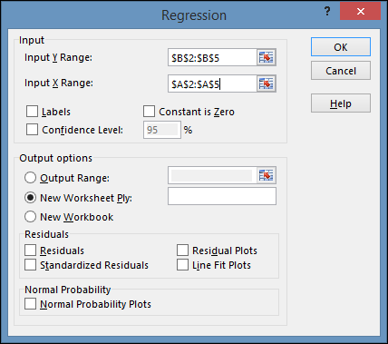
Step 4: Click ‘Ok’ to obtain the result.
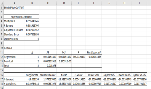
Hence, the obtained regression line is shown below:
Interpretation: Therefore, it can be concluded that the regression equation obtained by hand and software are approximately same.
Section 4:
To graph: A scatterplot which shows the fitting of least-squares regression line by software.
Section 4:
Explanation of Solution
Graph: Construct a scatterplot using excel as follows:
Step 1: Enter the data in Excel.
Step 2: Select the data. Click on Insert
Step 3: Now, put the cursor on the graph and a plus sign appears on the right hand side.
Step 4: Click on the plus sign and check the box for trend line.
Hence, the obtained graph is shown below:
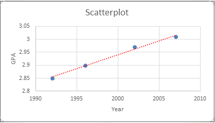
Interpretation: From the scatterplot, it can be seen that there is a linear dependency between GPA and year.
(c)
Section 1:
To find: The 95% confidence interval for the slope by hand.
(c)
Section 1:
Answer to Problem 30E
Solution: The confidence interval is
Explanation of Solution
Calculation: Now, compute
Year (x) |
GPA (y) |
|||
1992 |
2.85 |
2.852 |
0.000004 |
52.5625 |
1996 |
2.90 |
2.896 |
0.000016 |
10.5625 |
2002 |
2.97 |
2.962 |
0.000064 |
7.5625 |
2007 |
3.01 |
3.017 |
0.000049 |
60.0625 |
Now, compute the standard error of slope of regression
For 5% level of significance and
Compute the confidence interval as follows:
Interpretation: It can be said with 95% confidence that the GPA will increase between 0.008 and 0.014 over the time.
Section 2:
To find: The 95% confidence interval for the slope by software.
Section 2:
Answer to Problem 30E
Solution: The confidence interval is
Explanation of Solution
Calculation: Obtain the regression line using Excel as follows:
Step 1: Click on Data
Step 3: Enter Y variable and X variable input range.
Step 4: Click ‘Ok’ to obtain the result.
Hence, the obtained confidence interval for
Interpretation: Therefore, it can be concluded that the 95% confidence interval obtained by hand matched with the 95% confidence interval obtained by software.
Want to see more full solutions like this?
Chapter 10 Solutions
Introduction to the Practice of Statistics


 MATLAB: An Introduction with ApplicationsStatisticsISBN:9781119256830Author:Amos GilatPublisher:John Wiley & Sons Inc
 Probability and Statistics for Engineering and th...StatisticsISBN:9781305251809Author:Jay L. DevorePublisher:Cengage Learning
 Statistics for The Behavioral Sciences (MindTap C...StatisticsISBN:9781305504912Author:Frederick J Gravetter, Larry B. WallnauPublisher:Cengage Learning
 Elementary Statistics: Picturing the World (7th E...StatisticsISBN:9780134683416Author:Ron Larson, Betsy FarberPublisher:PEARSON
 The Basic Practice of StatisticsStatisticsISBN:9781319042578Author:David S. Moore, William I. Notz, Michael A. FlignerPublisher:W. H. Freeman
 Introduction to the Practice of StatisticsStatisticsISBN:9781319013387Author:David S. Moore, George P. McCabe, Bruce A. CraigPublisher:W. H. Freeman