Fluid Mechanics
8th Edition
ISBN: 9780073398273
Author: Frank M. White
Publisher: McGraw-Hill Education
expand_more
expand_more
format_list_bulleted
Videos
Textbook Question
Chapter 6, Problem 6.5P
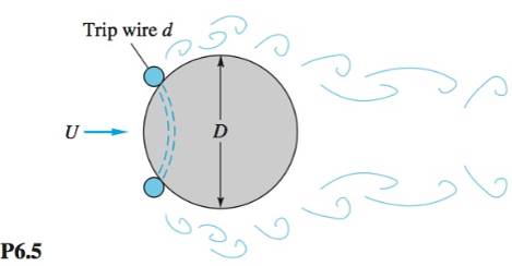
In flow past a body or wall, early transition to turbulence can be induced by placing a trip wire on the wall across the flow, as in Fig. P6.5. If the trip wire in Fig. P6.5 is placed where the local velocity is U, it will trigger turbulence if Ud/v = 850, where d is the wire diameter [3, p. 388]. If the sphere diameter is 20 cm and transition is observed at ReD = 90,000, what is the diameter of the trip wire in mm?
Expert Solution & Answer
Want to see the full answer?
Check out a sample textbook solution
Students have asked these similar questions
Air at 20⁰c and 1 ATM flows over a flat plate, v= 35 m/s.
The plate is 75 cm long and guarded at 60⁰c. Suppose the depth of one
Units on Z, count the transfer of Calor from that plate.
Pipelines are cleaned by pushing through them a closefitting cylinder called a pig . The name comes from thesquealing noise it makes sliding along. Reference 50describes a new nontoxic pig, driven by compressed air, forcleaning cosmetic and beverage pipes. Suppose the pigdiameter is 5-15/16 in and its length 26 in. It cleans a6-in-diameter pipe at a speed of 1.2 m/s. If the clearance isfi lled with glycerin at 20 8 C, what pressure difference, inpascals, is needed to drive the pig? Assume a linear velocityprofi le in the oil and neglect air drag.
How might the remarkable three-dimensional Taylorinstability of Fig. 4.14 be predicted? Discuss a generalprocedure for examining the stability of a given flowpattern.
Chapter 6 Solutions
Fluid Mechanics
Ch. 6 - Prob. 6.1PCh. 6 - The present pumping rate of crude oil through the...Ch. 6 - The Keystone Pipeline in the chapter opener photo...Ch. 6 - For flow of SAE 30 oil through a 5-cm-diameter...Ch. 6 - In flow past a body or wall, early transition to...Ch. 6 - P6.6 For flow of a uniform stream parallel to a...Ch. 6 - SAE 10W30 oil at 20°C flows from a tank into a...Ch. 6 - P6.8 When water at 20°C is in steady turbulent...Ch. 6 - A light liquid 950kg/m3 flows at an average...Ch. 6 - Water at 20°C flows through an inclined...
Ch. 6 - Water at 20°C flows upward at 4 m/s in a...Ch. 6 - Prob. 6.12PCh. 6 - Prob. 6.13PCh. 6 - Prob. 6.14PCh. 6 - Prob. 6.15PCh. 6 - Prob. 6.16PCh. 6 - P6.17 A capillary viscometer measures the time...Ch. 6 - P6.18 SAE 50W oil at 20°C flows from one tank to...Ch. 6 - Prob. 6.19PCh. 6 - The oil tanks in Tinyland are only 160 cm high,...Ch. 6 - Prob. 6.21PCh. 6 - Prob. 6.22PCh. 6 - Prob. 6.23PCh. 6 - Prob. 6.24PCh. 6 - Prob. 6.25PCh. 6 - Prob. 6.26PCh. 6 - Let us attack Prob. P6.25 in symbolic fashion,...Ch. 6 - Prob. 6.28PCh. 6 - Prob. 6.29PCh. 6 - Prob. 6.30PCh. 6 - A laminar flow element (LFE) (Meriam Instrument...Ch. 6 - SAE 30 oil at 20°C flows in the 3-cm.diametcr pipe...Ch. 6 - Prob. 6.33PCh. 6 - Prob. 6.34PCh. 6 - In the overlap layer of Fig. 6.9a, turbulent shear...Ch. 6 - Prob. 6.36PCh. 6 - Prob. 6.37PCh. 6 - Prob. 6.38PCh. 6 - Prob. 6.39PCh. 6 - Prob. 6.40PCh. 6 - P6.41 Two reservoirs, which differ in surface...Ch. 6 - Prob. 6.42PCh. 6 - Prob. 6.43PCh. 6 - P6.44 Mercury at 20°C flows through 4 m of...Ch. 6 - P6.45 Oil, SG = 0.88 and v = 4 E-5 m2/s, flows at...Ch. 6 - Prob. 6.46PCh. 6 - Prob. 6.47PCh. 6 - Prob. 6.48PCh. 6 - Prob. 6.49PCh. 6 - Prob. 6.50PCh. 6 - Prob. 6.51PCh. 6 - Prob. 6.52PCh. 6 - Water at 2OC flows by gravity through a smooth...Ch. 6 - A swimming pool W by Y by h deep is to be emptied...Ch. 6 - Prob. 6.55PCh. 6 - Prob. 6.56PCh. 6 - Prob. 6.57PCh. 6 - Prob. 6.58PCh. 6 - P6.59 The following data were obtained for flow of...Ch. 6 - Prob. 6.60PCh. 6 - Prob. 6.61PCh. 6 - Water at 20°C is to be pumped through 2000 ft of...Ch. 6 - Prob. 6.63PCh. 6 - Prob. 6.64PCh. 6 - Prob. 6.65PCh. 6 - Prob. 6.66PCh. 6 - Prob. 6.67PCh. 6 - Prob. 6.68PCh. 6 - P6.69 For Prob. P6.62 suppose the only pump...Ch. 6 - Prob. 6.70PCh. 6 - Prob. 6.71PCh. 6 - Prob. 6.72PCh. 6 - Prob. 6.73PCh. 6 - Prob. 6.74PCh. 6 - Prob. 6.75PCh. 6 - P6.76 The small turbine in Fig. P6.76 extracts 400...Ch. 6 - Prob. 6.77PCh. 6 - Prob. 6.78PCh. 6 - Prob. 6.79PCh. 6 - The head-versus-flow-rate characteristics of a...Ch. 6 - Prob. 6.81PCh. 6 - Prob. 6.82PCh. 6 - Prob. 6.83PCh. 6 - Prob. 6.84PCh. 6 - Prob. 6.85PCh. 6 - SAE 10 oil at 20°C flows at an average velocity of...Ch. 6 - A commercial steel annulus 40 ft long, with a = 1...Ch. 6 - Prob. 6.88PCh. 6 - Prob. 6.89PCh. 6 - Prob. 6.90PCh. 6 - Prob. 6.91PCh. 6 - Prob. 6.92PCh. 6 - Prob. 6.93PCh. 6 - Prob. 6.94PCh. 6 - Prob. 6.95PCh. 6 - Prob. 6.96PCh. 6 - Prob. 6.97PCh. 6 - Prob. 6.98PCh. 6 - Prob. 6.99PCh. 6 - Prob. 6.100PCh. 6 - Prob. 6.101PCh. 6 - *P6.102 A 70 percent efficient pump delivers water...Ch. 6 - Prob. 6.103PCh. 6 - Prob. 6.104PCh. 6 - Prob. 6.105PCh. 6 - Prob. 6.106PCh. 6 - Prob. 6.107PCh. 6 - P6.108 The water pump in Fig. P6.108 maintains a...Ch. 6 - In Fig. P6.109 there are 125 ft of 2-in pipe, 75...Ch. 6 - In Fig. P6.110 the pipe entrance is sharp-edged....Ch. 6 - For the parallel-pipe system of Fig. P6.111, each...Ch. 6 - Prob. 6.112PCh. 6 - Prob. 6.113PCh. 6 - Prob. 6.114PCh. 6 - Prob. 6.115PCh. 6 - Prob. 6.116PCh. 6 - Prob. 6.117PCh. 6 - Prob. 6.118PCh. 6 - Prob. 6.119PCh. 6 - Prob. 6.120PCh. 6 - Prob. 6.121PCh. 6 - Prob. 6.122PCh. 6 - Prob. 6.123PCh. 6 - Prob. 6.124PCh. 6 - Prob. 6.125PCh. 6 - Prob. 6.126PCh. 6 - Prob. 6.127PCh. 6 - In the five-pipe horizontal network of Fig....Ch. 6 - Prob. 6.129PCh. 6 - Prob. 6.130PCh. 6 - Prob. 6.131PCh. 6 - Prob. 6.132PCh. 6 - Prob. 6.133PCh. 6 - Prob. 6.134PCh. 6 - An airplane uses a pitot-static tube as a...Ch. 6 - Prob. 6.136PCh. 6 - Prob. 6.137PCh. 6 - Prob. 6.138PCh. 6 - P6.139 Professor Walter Tunnel needs to measure...Ch. 6 - Prob. 6.140PCh. 6 - Prob. 6.141PCh. 6 - Prob. 6.142PCh. 6 - Prob. 6.143PCh. 6 - Prob. 6.144PCh. 6 - Prob. 6.145PCh. 6 - Prob. 6.146PCh. 6 - Prob. 6.147PCh. 6 - Prob. 6.148PCh. 6 - Prob. 6.149PCh. 6 - Prob. 6.150PCh. 6 - Prob. 6.151PCh. 6 - Prob. 6.152PCh. 6 - Prob. 6.153PCh. 6 - Prob. 6.154PCh. 6 - Prob. 6.155PCh. 6 - Prob. 6.156PCh. 6 - Prob. 6.157PCh. 6 - Prob. 6.158PCh. 6 - Prob. 6.159PCh. 6 - Prob. 6.160PCh. 6 - Prob. 6.161PCh. 6 - Prob. 6.162PCh. 6 - Prob. 6.163PCh. 6 - Prob. 6.1WPCh. 6 - Prob. 6.2WPCh. 6 - Prob. 6.3WPCh. 6 - Prob. 6.4WPCh. 6 - Prob. 6.1FEEPCh. 6 - Prob. 6.2FEEPCh. 6 - Prob. 6.3FEEPCh. 6 - Prob. 6.4FEEPCh. 6 - Prob. 6.5FEEPCh. 6 - Prob. 6.6FEEPCh. 6 - Prob. 6.7FEEPCh. 6 - Prob. 6.8FEEPCh. 6 - Prob. 6.9FEEPCh. 6 - Prob. 6.10FEEPCh. 6 - Prob. 6.11FEEPCh. 6 - Prob. 6.12FEEPCh. 6 - Prob. 6.13FEEPCh. 6 - Prob. 6.14FEEPCh. 6 - Prob. 6.15FEEPCh. 6 - Prob. 6.1CPCh. 6 - Prob. 6.2CPCh. 6 - Prob. 6.3CPCh. 6 - Prob. 6.4CPCh. 6 - Prob. 6.5CPCh. 6 - Prob. 6.6CPCh. 6 - Prob. 6.7CPCh. 6 - Prob. 6.8CPCh. 6 - Prob. 6.9CPCh. 6 - A hydroponic garden uses the 10-m-long...Ch. 6 - It is desired to design a pump-piping system to...
Knowledge Booster


Learn more about
Need a deep-dive on the concept behind this application? Look no further. Learn more about this topic, mechanical-engineering and related others by exploring similar questions and additional content below.Similar questions
- Derive terminal velocity equations for disc shape particles starting from Eq.(6.33) for the following flow regimes: a) Stokes’ regime b) Newton’s regime c) Transition regime Diameter and length of the disc are dp and L=dp, respectivelyarrow_forwardWhen fluid in a long pipe starts up from rest at a uniformacceleration a , the initial flow is laminar. The flow undergoesa transition to turbulence at a time t * which depends, tofirst approximation, only upon a , ρ , and μ . Experiments by P. J. Lefebvre, on water at 20 8 C starting from rest with 1-gacceleration in a 3-cm-diameter pipe, showed transition att * = 1.02 s. Use this data to estimate ( a ) the transition timeand ( b ) the transition Reynolds number Re D for water flowaccelerating at 35 m/s 2 in a 5-cm-diameter pipe.arrow_forwardA force F = 1100 N pushes a piston of diameter 12 cmthrough an insulated cylinder containing air at 20 °C, as inFig. The exit diameter is 3 mm, and pa = 1 atm.Estimate (a) Ve, (b) Vp, and (c) m # e.arrow_forward
- P3.48 The small boat is driven at steady speed Vo by compressed air issuing from a 3-cm-diameter hole at Ve = 343 m/s and pe = 1 atm, Te = 30°C. Neglect air drag. The hull drag is kVo?, where k = 19 N · s/m². Estimate the boat speed Vo. %3D D= 3 cm Compressed V -E air Hull drag kVarrow_forwardSuppose that it is desired to estimate volume fl ow Q in apipe by measuring the axial velocity u ( r ) at specifi c points.For cost reasons only three measuring points are to be used.What are the best radii selections for these three points?arrow_forwardQ.5 A plate 1 mm distance from a fixed plate, is moving at 500 mm/s by a force induces a 2 shear stress of 0.3 kg(f)/m. The kinematic viscosity of the fluid (mass density 1000 kg/ 3. m) flowing between two plates (in Stokes) isarrow_forward
- Wall friction τ w , for turbulent flow at velocity U in apipe of diameter D , was correlated, in 1911, with a dimensionless correlation by Ludwig Prandtl’s studentH. Blasius: Suppose that ( ρ , U , μ , τ w ) were all known and it was desiredto find the unknown velocity U . Rearrange and rewritethe formula so that U can be immediately calculated.arrow_forwardThe drag of a sonar transducer is to be predicted, based on wind (Air) tunnel test data. The prototype is 1.5 m diameter sphere, is to be towed at 4.3 m/s in seawater. The model is 0.2 m diameter. Take: Air density = 1.2 kg/m, Air dynamic viscosity = 1.81 x 10$ Pa. s, seawater density = 1000 kg/m, seawater dynamic viscosity 1.813x 10 Pa s, If the drag of the model at these test conditions is 9.5 N, estimate the drag of the prototype in (N).arrow_forwardQ3) In some wind tunnels the test section is perforated to suck out fluid and provide a thin viscous boundary layer. The test section wall in Fig.3 contains 12064 holes of 5 mm diameter. The suction velocity through each hole is Vs = 8 m/s, and the test section entrance velocity is V₁ = 35 m/s. Assume incompressible steady flow of air at 20°C, compute, Vo, V₂ and Vf in m/s. Test section D₁ = 0.8 m Uniform suction D₁= 2.2 m Do = 2.5 m V₂ -L=4 m Fig.3 L Vo-arrow_forward
- A wind tunnel is used to measure the pressure distribution in the airflow over an airplane model. The air speed in the wind tunnel is low enough that compressible effects are negligible. The Bernoulli equation approximation is valid in such a flow situation everywhere except very close to the body surface or wind tunnel wall surfaces and in the wake region behind the model. Far away from the model, the air flows at speed V∞ and pressure P∞, and the air density ? is approximately constant. Gravitational effects are generally negligible in airflows, so we write the Bernoulli equation asP + 1/2 ρV2 = P∞ + 1/2 ρV2∞ Nondimensionalize the equation, and generate an expression for the pressure coefficient Cp at any point in the flow where the Bernoulli equation is valid. Cp is defined as Cp = P−P∞/1/2ρV2arrow_forwardFrom the laminar boundary layer the velocity distributions given below, find the momentum thickness θ, boundary layer thickness δ, wall shear stress τw, skin friction coefficient Cf , and displacement thickness δ*1. A linear profile, u(x, y) = a + by 2. von K ́arm ́an’s second-order, parabolic profile,u(x, y) = a + by + cy2 3. A third-order, cubic function,u(x, y) = a + by + cy2+ dy3 4. Pohlhausen’s fourth-order, quartic profile,u(x, y) = a + by + cy2+ dy3+ ey4 5. A sinusoidal profile,u = U sin (π/2*y/δ)arrow_forwardThe traditional "Moody-type" pipe friction correlation in Chap. 6 is of the form 2APD f = pVL (pVD и "D, where D is the pipe diameter, L the pipe length, and e the wall roughness. Note that pipe average velocity V is used on both sides. This form is meant to find Ap when V is known. (a) Suppose that Ap is known, and we wish to find V. Rearrange the above function so that V is isolated on the left-hand side. Use the following data, for e/D = 0.005, to make a plot of your new function, with your velocity parameter as the ordinate of the plot. 0.0356 | 0.0316 | 0.0308 pVD/u | 15,000 | 75,000 | 250,000 | 900,000 | 3,330,000 0.0305 0.0304 (b) Use your plot to determine V, in m/s, for the following pipe flow: D = 5 cm, e = 0.025 cm, L = 10 m, for water flow at 20°C and 1 atm. The pressure drop Ap is 110 kPa.arrow_forward
arrow_back_ios
SEE MORE QUESTIONS
arrow_forward_ios
Recommended textbooks for you
 Elements Of ElectromagneticsMechanical EngineeringISBN:9780190698614Author:Sadiku, Matthew N. O.Publisher:Oxford University Press
 Mechanics of Materials (10th Edition)Mechanical EngineeringISBN:9780134319650Author:Russell C. HibbelerPublisher:PEARSON
 Thermodynamics: An Engineering ApproachMechanical EngineeringISBN:9781259822674Author:Yunus A. Cengel Dr., Michael A. BolesPublisher:McGraw-Hill Education
 Control Systems EngineeringMechanical EngineeringISBN:9781118170519Author:Norman S. NisePublisher:WILEY
 Mechanics of Materials (MindTap Course List)Mechanical EngineeringISBN:9781337093347Author:Barry J. Goodno, James M. GerePublisher:Cengage Learning
 Engineering Mechanics: StaticsMechanical EngineeringISBN:9781118807330Author:James L. Meriam, L. G. Kraige, J. N. BoltonPublisher:WILEY
Elements Of Electromagnetics
Mechanical Engineering
ISBN:9780190698614
Author:Sadiku, Matthew N. O.
Publisher:Oxford University Press
Mechanics of Materials (10th Edition)
Mechanical Engineering
ISBN:9780134319650
Author:Russell C. Hibbeler
Publisher:PEARSON
Thermodynamics: An Engineering Approach
Mechanical Engineering
ISBN:9781259822674
Author:Yunus A. Cengel Dr., Michael A. Boles
Publisher:McGraw-Hill Education
Control Systems Engineering
Mechanical Engineering
ISBN:9781118170519
Author:Norman S. Nise
Publisher:WILEY
Mechanics of Materials (MindTap Course List)
Mechanical Engineering
ISBN:9781337093347
Author:Barry J. Goodno, James M. Gere
Publisher:Cengage Learning
Engineering Mechanics: Statics
Mechanical Engineering
ISBN:9781118807330
Author:James L. Meriam, L. G. Kraige, J. N. Bolton
Publisher:WILEY
Intro to Compressible Flows — Lesson 1; Author: Ansys Learning;https://www.youtube.com/watch?v=OgR6j8TzA5Y;License: Standard Youtube License