
Concept explainers
Videos
The following equations define the concentrations of threereactants:
If the initial conditions are
To calculate: The concentration for the times from
Initials conditions are
Answer to Problem 7P
Solution:
The concentration of the reactants
The concentration of the reactants
The concentration of the reactants
The concentration of the reactants
Explanation of Solution
Given information:
The system of equations,
Initial conditions,
Formula used:
To calculate the values of
Eigen value
Calculation:
Consider the system of first order nonlinear differential equation of reactants
To calculate equilibrium points, consider the equations given below:
Compare the system of first order nonlinear differential equations with the above equations,
Therefore, the equilibrium point is,
Suppose, the system of non-linear differential equations are equal to some functions, that is,
Now, compare these equations with system of non-linear differential equations,
Now, find the Jacobian matrix,
Then, the Jacobian matrix at the equilibrium points
Now, the linearized system corresponding to nonlinear system of differential equation is,
Let,
Suppose,
Thus,
Now calculate the determinant as,
Therefore, the eigenvalues of the matrix are
Now, find the eigenvector corresponding to each eigenvalue of the matrix.
The eigenvector is,
Where,
Substitute the value of X in
Put
Put
Put
Therefore, the eigenvector corresponding to each eigenvalue of the matrix are respectively
Hence, the solution of the system of nonlinear differential equation is,
After solve the above equation,
Then the values of
The initial conditionsgiven as,
Now, apply the initial condition in the above equations,
This imply that,
Then,
Substitute, the value of
The concentration at
Therefore, theconcentration of the reactants
Now, the concentration at
Therefore, the concentration of the reactants
Now, the concentration at
Therefore, the concentration of the reactants
Now, the concentration at
Use the following MATLAB code to plot the concentrationvalues,
Execute the above to obtain the plot as,
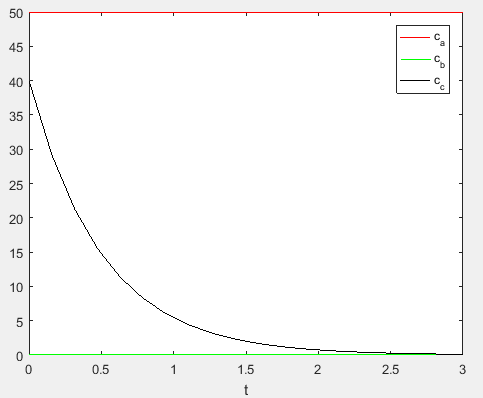
Therefore, the concentration of the reactants
Hence, the concentration of the reactants
Want to see more full solutions like this?
Chapter 28 Solutions
Numerical Methods for Engineers


- Show that r : y= 3. 2narrow_forwardA chemist creates 200 milliliters of a 52.5 % alcohol solution by combining a 30 % alcohol solution with a 75 % alcohol solution. If x represents the amount of the 30 % alcohol solution used and y represents the amount of the 75 % alcohol solution used, which of the following could be used to model the given infromation? 200 0.32+ 0.3x + 0.75y 105 + 200 %3D 0.03x + 0.075y 105 200 3x + 7.5y 105 200 0.3x 0.75y 52.5 %3D + 200 %3D O 30z + 75y 52.5arrow_forwardEliminate the arbitrary constant in the equation y? = 4ax. a. x?dy + 2xydx = 0 b. x²dy – 2xydx = 0 c. y?dx + 2xydy = 0 d. y?dx – 2xydy = 0 %3D -arrow_forward
 College AlgebraAlgebraISBN:9781305115545Author:James Stewart, Lothar Redlin, Saleem WatsonPublisher:Cengage Learning
 Algebra and Trigonometry (MindTap Course List)AlgebraISBN:9781305071742Author:James Stewart, Lothar Redlin, Saleem WatsonPublisher:Cengage Learning
 Calculus For The Life SciencesCalculusISBN:9780321964038Author:GREENWELL, Raymond N., RITCHEY, Nathan P., Lial, Margaret L.Publisher:Pearson Addison Wesley,