
Excel Applications for Accounting Principles
4th Edition
ISBN: 9781111581565
Author: Gaylord N. Smith
Publisher: Cengage Learning
expand_more
expand_more
format_list_bulleted
Videos
Textbook Question
Chapter 15, Problem 2R
The comparative financial statements of Global Technology are as follows:
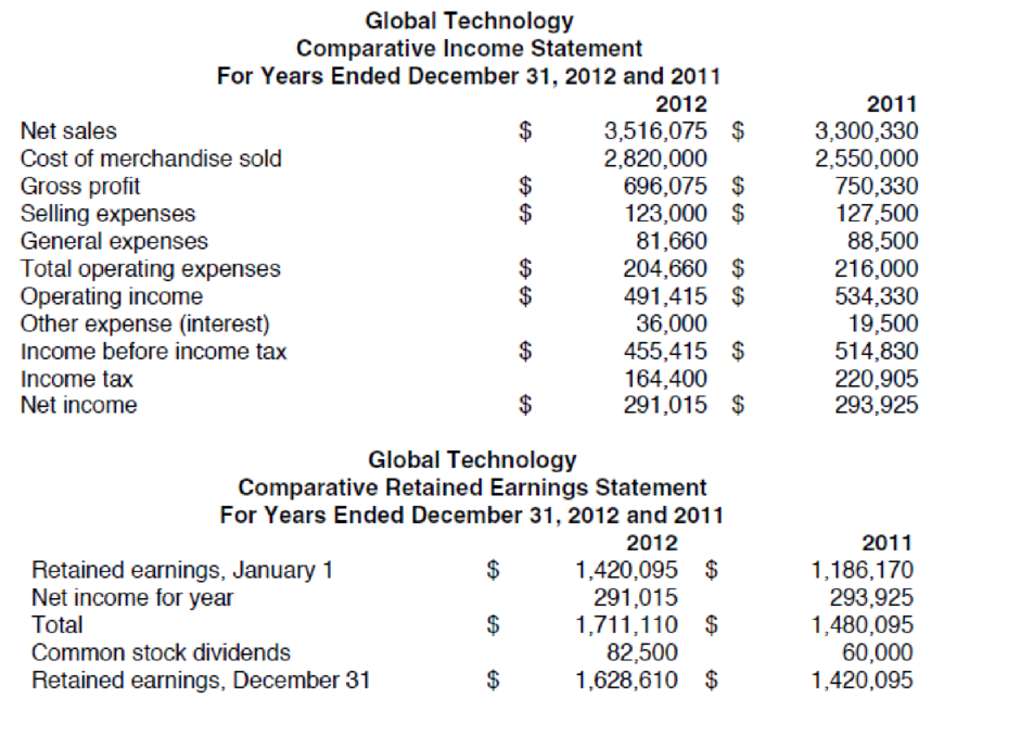
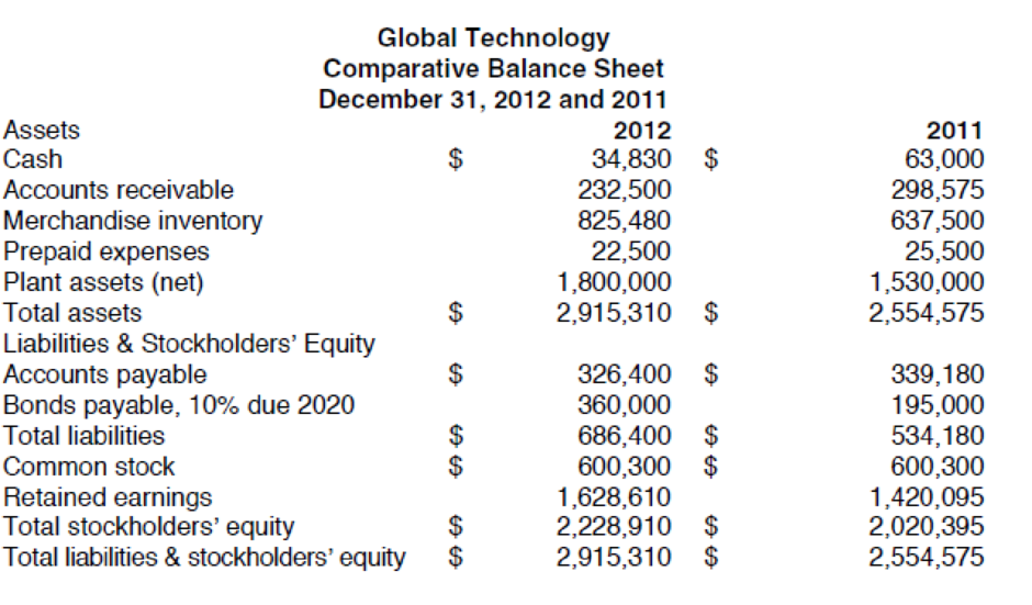
Open the file RATIOA from the website for this book at cengagebrain.com. Enter the formulas in the appropriate cells. Enter your name in cell A1. Save the completed model as RATIOA2. Print the worksheet when done. Also print your formulas. Check figure: Acid test (quick) ratio (cell C58), .82.
Expert Solution & Answer
Want to see the full answer?
Check out a sample textbook solution
Students have asked these similar questions
Application Time! 1) You will type the TVM inputs in the table provided from the "Info Sheet". 2)
Mirror the inputs from the "Info Sheet" to the TVM cells provided. 3) Within the TVM cells, if needed,
compound. 4) In the "ANSWER" cell show us your TVM calculation.
Goal 1: Opened an account with $1500, with the hope to have a total of $2500 saved in an
LG2-Q8 emergency fund within one year (no additional payments).
What would the quarterly interest rate be needed to reach this goal?
Goal 2: A credit card balance of $2000 with an 15% rate. The goal is to pay off the credit card
LG2-Q9 by the end of the year. (future is a $0 balance)
What would be the monthly payment to reach this goal?
Goal 3: Student loan balance of $18,000 at 6.5% and making $425 monthly payments. (future
LG2-Q10 is a $0 balance)
How many months will it take to complete this goal?
in fuo (no
Compounding Number
(select from dropdown)
4
Compounding Number
(select from dropdown)
12
Compounding Number
(select from…
Using Excel, create a table that shows the relationship between the interestearned and the amount deposited, as shown. we will first create the dollar amount column and the interest row, as shown . Next we will type into cell B3 the formula = $A3*B$2. We can now use the Fill command to copy the formula in other cells, resulting in the table as shown. Note that the dollar sign before A3 means column A is to remain unchanged in the calculations when the formula is copied into other cells. Also note that the dollar sign before 2 means that row 2 is to remain unchanged in calculations when the Fill command is used.
Further info is in the attached images
For the Excel part of the question give the solutions in the form of the Excel equations. Please and thank you! :)
Download the Applying Excel form and enter formulas in all cells that contain question marks.
For example, in cell B34 enter the formula "= B9".
After entering formulas in all of the cells that contained question marks, verify that the dollar amounts match the example in the text.
Check your worksheet by changing the beginning work in process inventory to 100 units, the units started into production during the period to 2,500 units, and the units in ending work in process inventory to 200 units, keeping all of the other data the same as in the original example. If your worksheet is operating properly, the cost per equivalent unit for materials should now be $152.50 and the cost per equivalent unit for conversion should be $145.50.
Thank you!
Chapter 15 Solutions
Excel Applications for Accounting Principles
Ch. 15 - The comparative financial statements of Global...Ch. 15 - The comparative financial statements of Global...Ch. 15 - a. What information does a comparison of the...Ch. 15 - Prepare a ratio analysis for Global Technology for...Ch. 15 - Compare your printout from requirement 2 with your...Ch. 15 - With the 2013 data still on the screen, click the...
Knowledge Booster


Learn more about
Need a deep-dive on the concept behind this application? Look no further. Learn more about this topic, accounting and related others by exploring similar questions and additional content below.Similar questions
- The general ledger of Jay Consulting shows the following balances at July 31: Jay has asked you to develop a worksheet that will serve as a trial balance (file name PTB). Use the data provided as input for your model. Review the Model-Building Problem Checklist on page 154 to ensure that your worksheet is complete. Print the worksheet when done. Check figure: Total debits, 17,731. To test your model, use the following balances at August 31: Print the worksheet when done. Check figure: Total debits, 18,810. CHART (optional) Using the test data worksheet, prepare a pie chart showing the percentage of each asset to total assets. Print the chart when done.arrow_forwardCreate a Balance Sheet for Till La Hok Computer Services. The other picture is just for the format .arrow_forwardRequired information (The Excel worksheet form that appears below is to be used to recreate part of the example relating to Turbo Crafters that appears earlier in the chapter.) Download the Applying Excel form and enter formulas in all cells that contain question marks. For example, in cell B13 enter the formula "= B5". After entering formulas in all of the cells that contained question marks, verify that the dollar amounts match the example in the text. Check your worksheet by changing the estimated total amount of the allocation base in the Data area to 50,000 machine-hours, keeping all of the other data the same as in the original example. If your worksheet is operating properly, the predetermined overhead rate should now be $6.00 per machine-hour. If you do not get this answer, find the errors in your worksheet and correct them. Save your completed Applying Excel form to your computer and then upload it here by clicking "Browse." Next, click "Save." You will use this…arrow_forward
- Please note: You can draw your trees either by hand on paper or in Excel. If you do it on a paper, please take a picture of the tree and insert it in your solution file. You can submit your solution as an Excel file or Word document. In either case, your solution should contain your decision trees and all necessary calculations (not just the results of calculations). Problem 1. The WHN Company Problem. The WHN Company is going to introduce one of the three new products: a widget, a hummer, or a nimnot. The market condition could be favorable, stable, or unfavorable with the probabilities 0.2, 0.5, and 0.3 respectively. The monetary outcomes for each product under each condition are described in the following table: Unfavorable $120,000 $70,000 -875,000 $40,000 $20,000 $30,000 $30,000 Favorable Stable Widget Hummer $60,000 Nimnot $35,000 Create a decision tree to identify which new product should be introduced in order to maximize the company's profit?arrow_forwardFor the following five spreadsheet functions, (a) write the values of the engineering economy symbols P, F, A, i, and n, using a ? for the symbol that is to be determined, and (b) state whether the displayed answer will have a positive sign, a negative sign, or it can’t be determined from the entries. (1) = FV(8%, 10, 3000, 8000) (2) = PMT(12%, 20, –16000) (3) = PV(9%, 15, 1000,600) (4) = NPER(10%, –290,, 12000) (5) = FV(5%, 5, 500, –2000)arrow_forwardWork the problem out by hand on a piece of paper so that you know what the answers should be. All dollar amounts (except EPS) should end in ",000" The schedule and statment in your output should compute mathematically from TOP to Bottom, so check and make sure that's the case Math Example: If A - B = C, then A - C = B and A = B + C Prepare an output section that produces the following items: 1) "COGS Schedule", 2) "Income Statement", and 3) "Retained Earning Statement". The reporting period is for the calendar year of 2023. The output items should be placed on a separate 'sheet' (the heading "... OUTPUT SECTION ..." should be centered over all columns to which it relates: [A1..G1]). Naming of the output 'sheet' should be "OUTPUT". No number (dollar amount, shares, or percentage) or company name should be typed (hard coded) directly into any cell in the output section, as this would prevent your output from being correct when the input is changed. Instead, the output section must…arrow_forward
- 1. Choose three of the following five technologies/techniques and explain why you think it is helpful in accounting analytics based on your lab experience in this course. Use some examples in your explanation. Limit your answer to 500 words in total. A. XBRL B. Tableau C. VLOOKUP function D. Pivot table E. Regressionarrow_forwardPlease match the answer to the answe in green box in the image. Please answer step by step how you got all the numbers and the calculations you did provide in detail.arrow_forwardPart B: Calculate FV or PV for the following questions and put all in the format uploaded in the Moodle: (Put any number you want in the empty places and then calculate)arrow_forward
- What are the Microsoft Excel formulaues used to input these? Is there a way to show each formula for how you came up with these. Not just the ratios but what you would input into excel that would automatically calculate the correct answers?arrow_forwardYou wish to create a Data Table that calculates the NPV with various initial outlays in D1:E6. Which cell should be entered into the Data Table dialog box, and in which edit box?arrow_forwardYou are provided with the following information. Please give me the answers in an excel format.arrow_forward
arrow_back_ios
SEE MORE QUESTIONS
arrow_forward_ios
Recommended textbooks for you
 Excel Applications for Accounting PrinciplesAccountingISBN:9781111581565Author:Gaylord N. SmithPublisher:Cengage Learning
Excel Applications for Accounting Principles
Accounting
ISBN:9781111581565
Author:Gaylord N. Smith
Publisher:Cengage Learning
Topic 6 - Financial statement analysis; Author: drdavebond;https://www.youtube.com/watch?v=uUnP5qkbQ20;License: Standard Youtube License