
Videos
A machine that grinds valves is set to produce valves whose lengths have
- a. Find the rejection region if the test is made at the 5% level.
- b. Find the rejection region if the test is made at the 10% level.
- c. If the sample mean length is 99.97 mm, will H0 be rejected at the 5% level?
- d. If the sample mean length is 100.01 mm, will H0 be rejected at the 10% level?
- e. A critical point is 100.015 mm. What is the level of the test?
a.
Find the rejection region, if the test is made at 5% level.
Answer to Problem 11SE
The null hypothesis will be rejected, if
Explanation of Solution
Given info:
The hypotheses are:
The standard deviation is 0.1 mm and the sample size is 100.
Calculation:
Under
The rejection region consists of lower and upper 2.5% of the null distribution because the alternative hypothesis is of the form is
The lower and upper boundary is calculated as follows:
Software Procedure:
Step-by-step procedure to obtain the 5th percentile using the MINITAB software:
- Choose Graph > Probability Distribution Plot choose View Probability > OK.
- From Distribution, choose ‘Normal’ distribution.
- Click the Shaded Area tab.
- Choose Probability Value and Both Tails for the region of the curve to shade.
- Enter the Probability value as 0.05.
- Click OK.
Output using the MINITAB software is given below:
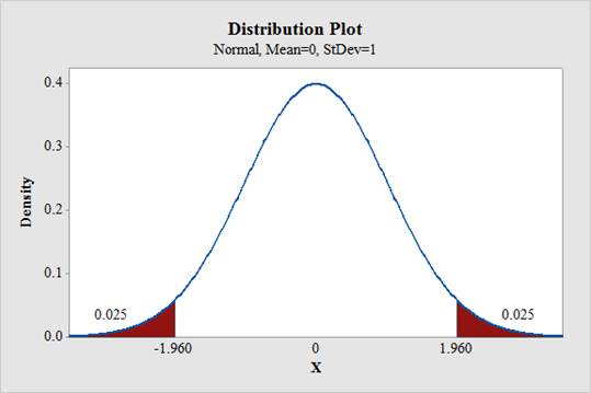
Therefore, the z-sore corresponding to the lower and upper 2.5% is –1.96 and +1.96, respectively.
The boundaries are calculated as follows:
Lower boundary:
Upper boundary:
Therefore, the rejection region is
If
b.
Find the rejection region, if the test is made at 10% level.
Answer to Problem 11SE
The null hypothesis will be rejected, if
Explanation of Solution
Calculation:
The rejection region consists of lower and upper 5% of the null distribution because the alternative hypothesis is of the form is
The lower and upper boundary is calculated as follows:
Software Procedure:
Step-by-step procedure to obtain the 10th percentile using the MINITAB software:
- Choose Graph > Probability Distribution Plot choose View Probability > OK.
- From Distribution, choose ‘Normal’ distribution.
- Click the Shaded Area tab.
- Choose Probability Value and Both Tails for the region of the curve to shade.
- Enter the Probability value as 0.10.
- Click OK.
Output using the MINITAB software is given below:
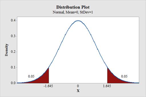
Therefore, the z-sore corresponding to the lower and upper 5% is –1.645 and +1.645, respectively.
The boundaries are calculated as follows:
Lower boundary:
Upper boundary:
Therefore, the rejection region is
If
c.
Check whether the null hypothesis will be rejected at the 5% level, if the sample mean length is 99.97 mm.
Answer to Problem 11SE
Yes, the null hypothesis will be rejected at 5% level.
Explanation of Solution
Calculation:
From part a., the null hypothesis will be rejected, if
Here, the sample mean is 99.97 mm.
Thus, the null hypothesis will be rejected at 5% level because
d.
Check whether the null hypothesis will be rejected at the 10% level, if the sample mean length is 100.01 mm.
Answer to Problem 11SE
No, the null hypothesis will not be rejected at 10% level.
Explanation of Solution
Calculation:
From part b., the null hypothesis will be rejected, if
Here, the sample mean is 100.01 mm.
Therefore, the null hypothesis will not be rejected at 10% level because
d.
Find the level of the test, if the critical point is 100.015 mm.
Answer to Problem 11SE
The level is 0.1336.
Explanation of Solution
Calculation:
Type-1 error: Rejecting the null hypothesis
The alternative hypothesis is of the form is
The given critical point is 100.015 mm and the other critical point is
The level of the test is,
The z-score of 99.985 is calculated below:
Software Procedure:
Step-by-step procedure to obtain the
- Choose Graph > Probability Distribution Plot choose View Probability > OK.
- From Distribution, choose ‘Normal’ distribution.
- Click the Shaded Area tab.
- Choose X Value and Left Tail for the region of the curve to shade.
- Enter the data value as -1.5.
- Click OK.
Output using the MINITAB software is given below:
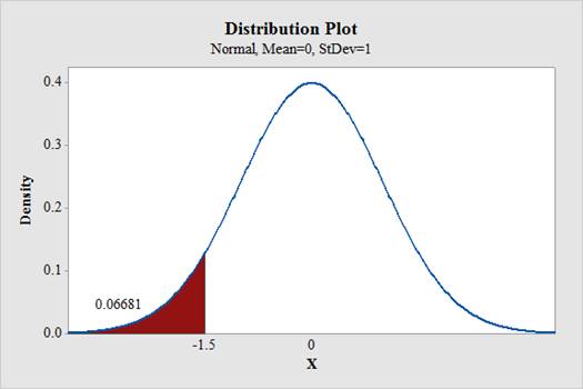
Thus,
The z-score of 100.015 is calculated below:
Software Procedure:
Step-by-step procedure to obtain the
- Choose Graph > Probability Distribution Plot choose View Probability > OK.
- From Distribution, choose ‘Normal’ distribution.
- Click the Shaded Area tab.
- Choose X Value and Right Tail for the region of the curve to shade.
- Enter the data value as 1.5.
- Click OK.
Output using the MINITAB software is given below:
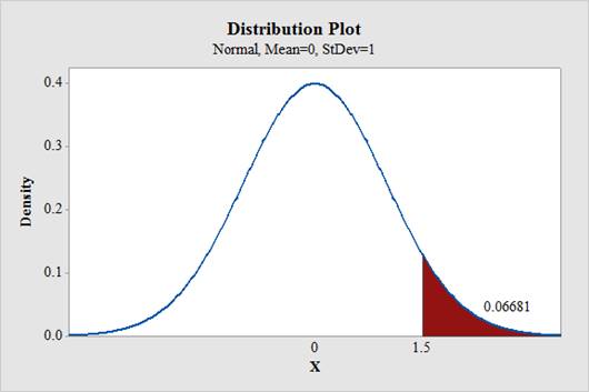
From the output,
Therefore, the level is given below:
Thus, the level is 0.1336.
Want to see more full solutions like this?
Chapter 6 Solutions
Statistics for Engineers and Scientists
Additional Math Textbook Solutions
Applied Statistics in Business and Economics
Elementary Statistics: Picturing the World (7th Edition)
Statistics for Psychology
Basic Business Statistics, Student Value Edition (13th Edition)
Intro Stats, Books a la Carte Edition (5th Edition)


 Glencoe Algebra 1, Student Edition, 9780079039897...AlgebraISBN:9780079039897Author:CarterPublisher:McGraw Hill
 Big Ideas Math A Bridge To Success Algebra 1: Stu...AlgebraISBN:9781680331141Author:HOUGHTON MIFFLIN HARCOURTPublisher:Houghton Mifflin Harcourt