
Concept explainers
Videos
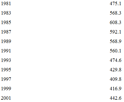
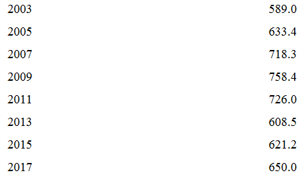
Military spending: The following table presents the amount spent, in billions of dollars, on national defense by the U.S. government every other year for the years 1951 through 2017. The amounts are adjusted for inflation, and represent 2017 dollars.
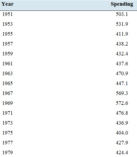
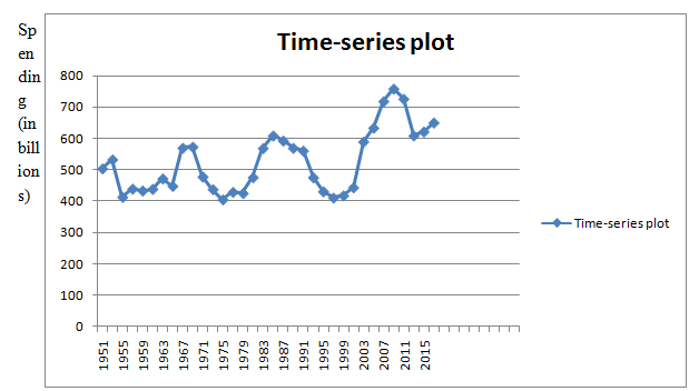
- Construct a time-series plot for these data.
- The plot covers seven decades, from the 1950s through the period 2010—2017. During which of these decades did national defense spending increase, and during which decades did it decrease?
- The United States fought in the Korean War, which ended in 1953. What effect did the end of the war have on military spending after 1953?
- During the period 1965—1963, the United States steadily increased the number of troops in Vietnam from 23,000 at the beginning of 1965 to 537.000 at the end of 1968.
Beginning in 1969, the number of Americans in Vietnam was steadily reduced, with the last of them leaving in 1975. How is this reflected in the national defense spending from 1965 to 1975?
a.
To construct:A time-series plot of the given data.
Explanation of Solution
Given information:
The dataset:
| Year | Spending |
| 1951 | 503.1 |
| 1953 | 531.9 |
| 1955 | 411.9 |
| 1957 | 438.2 |
| 1959 | 432.4 |
| 1961 | 437.6 |
| 1963 | 470.9 |
| 1965 | 447.1 |
| 1967 | 569.3 |
| 1969 | 572.6 |
| 1971 | 476.8 |
| 1973 | 436.9 |
| 1975 | 404.0 |
| 1977 | 427.9 |
| 1979 | 424.4 |
| 1981 | 475.1 |
| 1983 | 568.3 |
| 1985 | 608.3 |
| 1987 | 592.1 |
| 1989 | 568.9 |
| 1991 | 560.1 |
| 1993 | 474.6 |
| 1995 | 429.8 |
| 1997 | 409.8 |
| 1999 | 416.9 |
| 2001 | 442.6 |
| 2003 | 589.0 |
| 2005 | 633.4 |
| 2007 | 718.3 |
| 2009 | 758.4 |
| 2011 | 726.0 |
| 2013 | 608.5 |
| 2015 | 621.2 |
| 2017 | 650.0 |
Graph:
A time-series plot for the given data is given by
b.
To find:The decade during which the national defence spending increasing and the decade during which the national defence spending increasing.
Answer to Problem 27E
The trend in the vacancy rate during the time period from 2012 to 2015 is decreasing.
Explanation of Solution
Solution:
A time-series plot for the given data is given by
From the time-series plot, we can see that during 1960s, 1980s and 2000s, the national defence spending is increasing and during 1950s, 1970s, 1990s and 2010s, the national defence spending is decreasing
Hence,
Increased decade: 1960s, 1980s and 2000s
Decreased decade: 1950s, 1970s, 1990s and 2010s.
c.
To find: The effects of the end of the war have on military spending after 1953.
Answer to Problem 27E
The effects of the end of the war have on military spending after 1953 is that it caught a big decrease.
Explanation of Solution
Solution:
A time-series plot for the given data is given by
From the time-series plot, we can see that after 1953, there was causing a big decrease in the military spending. The military spending was falling from 531.9 to 411.9 during 1953-1955.
Hence, the effects of the end of the war have on military spending after 1953 is that there caused a big decrease.
d.
To explain: The reflection in the national defence spending from 1965 to 1975.
Answer to Problem 27E
The national defence spending is increased from 1965 to 1969 and then decreased from 1969 to 1975.
Explanation of Solution
Given information: The following table presents the amount spent, in billions of dollars, on national defence by the U.S. government every other year for the years 1951 through 2017. The amounts are adjusted for inflation, and represent 2017 dollars.
| Year | Spending |
| 1951 | 503.1 |
| 1953 | 531.9 |
| 1955 | 411.9 |
| 1957 | 438.2 |
| 1959 | 432.4 |
| 1961 | 437.6 |
| 1963 | 470.9 |
| 1965 | 447.1 |
| 1967 | 569.3 |
| 1969 | 572.6 |
| 1971 | 476.8 |
| 1973 | 436.9 |
| 1975 | 404.0 |
| 1977 | 427.9 |
| 1979 | 424.4 |
| 1981 | 475.1 |
| 1983 | 568.3 |
| 1985 | 608.3 |
| 1987 | 592.1 |
| 1989 | 568.9 |
| 1991 | 560.1 |
| 1993 | 474.6 |
| 1995 | 429.8 |
| 1997 | 409.8 |
| 1999 | 416.9 |
| 2001 | 442.6 |
| 2003 | 589.0 |
| 2005 | 633.4 |
| 2007 | 718.3 |
| 2009 | 758.4 |
| 2011 | 726.0 |
| 2013 | 608.5 |
| 2015 | 621.2 |
| 2017 | 650.0 |
During the period 1965-1968, the United States steadily increased the number of troops in Vietnam from 23,000 at the beginning of 1965 to 537,000 at the end of 1968. Beginning in 1969, the number of Americans in Vietnam was steadily reduced, with the last of themleaving in 1975.
A time-series plot for the given data is given by
From 1965 to 1975, the national defence spending is increasing from 1965 to 1969 and then decreasing from 1969 to 1975.
Hence, the national defence spending is increased from 1965 to 1969 and then decreased from 1969 to 1975.
Want to see more full solutions like this?
Chapter 2 Solutions
Elementary Statistics ( 3rd International Edition ) Isbn:9781260092561


- Table 6 shows the year and the number ofpeople unemployed in a particular city for several years. Determine whether the trend appears linear. If so, and assuming the trend continues, in what year will the number of unemployed reach 5 people?arrow_forwardA time series plot showing the national murder rates per 100,000 people in the United States for the years 1990 to 2010 is shown below. Approximate the change in homicide rate from 2000 to 2010. National Homicide Rates, United States Homicide rate per 100,000 people 10 6 8 7 9 С & 1990 Select one: Oa. -0.4 O b. -0.7 C. -1 d. -1.2 1992 Clear my choice 1994 1996 1998 2000 2002 2004 2006 2008 Year 2010arrow_forwardIn retail, a store manager uses time series models to understand shopping trends. Review the scatter plot of the store’s sales from 2010 through 2021 to answer the questions. See attached as image. Here is the data for Fiscal Year and Sales: Fiscal Year Sales 2010 $260,123.00 2011 $256,853.00 2012 $274,366.00 2013 $290,525.00 2014 $322,318.00 2015 $380,921.00 2016 $541,925.00 2017 $909,050.00 2018 $1,817,521.00 2019 $3,206,564.00 2020 $4,921,005.00 2021 $5,686,338.00 Time series decomposition seeks to separate the time series (Y) into 4 components: trend (T), cycle (C), seasonal (S), and irregular (I). What is the difference between these components? The model can be additive or multiplicative. When do you use each? Review the scatter plot of the exponential trend of the time series data. Do you observe a trend? If so, what type of trend do you observe? What predictions might you make about the store’s annual sales over the next few years?arrow_forward
- the table shows the percent of households with internet access for selected years from 2009 and projected through 2015. Year Percent of households 2009 67 2010 70 2011 72.5 2012 75 2013 76.5 2014 77.2 2015 78 Use the model to predict the percent of households with internet access in 2022.arrow_forwardThe following graph shows the annual number of car accidents in California. Which of the following statements about the annual number of car accidents is an accurate conclusion? Yearly Car Accidents 180,000 160,000 140,000 120,000 100,000 80,000 60,000 40,000 20,000 2000 2005 Year 1985 1990 1995 2010 2015 2020 e 2018 Glynlyon, Inc. O There is a greater decrease in the annual number of car accidents from 1994 to 1995 than from 1997 to 1998. O There is a smaller decrease in the annual number of car accidents from 1999 to 2000 than from 1997 to 1998. O There is a smaller increase in the annualnumber of car accidents from 1995 to 1996 than from 1998 to 1999. O There is a greater increase in the annual number of car accidents from 1993 to 1994 than from 1996 to 1997. Car Accidentsarrow_forwardFrom the data given below, find the second five years moving average. Year Sales 2012 20 2013 25 2014 30 2015 35 2016 40 2017 45 2018 50arrow_forward
- B4. A company has collected and smoothened its historical yearly sales data of a product from 2015 up to 2021. The following table shows the sales and moving average figures. Sales Three-year moving avcrage Year Five-ycar moving avcrage (S thousands) 2015 2016 326.0 324.0 E 367.4 2017 344.0 2018 383.0 371.0 2019 B. 389.0 2020 398.0 D 2021 428.0 Calculate the missing values of4, B, C, D. E and F(Correct to I decimal place). B5. A lottery consists of 49 balls numbered 1 through 49 and 6 of them are drawn at random. (a) You can pick 6 different numbers for a betting ticket. How many selections are possible? (b) If prizes will be paid to those picking 4 to 6 drawn numbers, how many winning selections are possible? రarrow_forwardCryptocurrencies have rapidly become an important alternative to traditional currencies for many types of transactions. Etherium, one of the most prominent cryptocurrencies, has rapidly appreciated in value. Daily Etherium trading information for the first 332 days of 2021. It includes the following variables: Date Day – Day of the year, used to assess trend over time Volume (US $) – Daily trading volume Opening Price (US $) – Opening price for daily trading Price Change (US $) – Daily change in price from opening to close 1. Determine the sample correlation coefficient, r, between Volume and Price Change. Test the alternative hypothesis that Volume has a linear relationship to Price Change. Specifically, what are the test statistic and the p-value for that test statistic? For α = .05, what do you conclude about the relationship between the variables? (reminder: the T.DIST.2T function requires input of a positive test statistic)arrow_forwardSuppose a man invested $250 at the end of 1900 in each of three funds that tracked the averages of stocks, bonds, and cash, respectively. Assuming that his investments grew at the rates given in the table to the right, approximately how much would each investment have been worth at the end of 2007? His investment in the fund tracking stocks would be worth approximately $. (Do not round until the final answer. Then round to two decimal places as needed.) Category Stocks Bonds Cash Average Annual Return 6.7% 2.4% 0.7%arrow_forward
- The following chart shows "living wage" jobs in Rochester per 1000 working age adults over a 5 year period. Year 2016 2017 2018 2019 2020 Jobs 675 730 775 805 820 What is the average rate of change in the number of living wage jobs from 2016 to 2018? Jobs/Year What is the average rate of change in the number of living wage jobs from 2018 to 2020? Jobs/Yeararrow_forwardThe table shows the inflation-adjusted annual income per person in 1990 and 2011 for each listed country. Which country had the smallest relative increase in annual income per person from 1990 to 2011? What was the smallest relative increase? |1990 2011 |Country A $33,304 $41,451 Country B $23,036 $30,829 Country C $1,986 $7,656 Country D $893 $1,140 Country had the smallest relative increase in annual income per person from 1990 to 2011. It was about %. (Round to the nearest tenth as needed.)arrow_forwardThe total amount of consumer credit has been increasing steadily in recent years. The following table gives the total outstanding consumer credit (in billions of dollars). Answer parts (a) through (e) below. Year 2004 2005 2006 2007 2008 Consumer Credit 2210.5 2303.8 2437.0 2517.9 2595.1 Year 2009 2010 2011 2012 2013 The consumer credit is growing about $ (Round to two decimal places as needed.) *** Consumer Credit 2557.5 2648.1 2756.0 2926.3 3099.2 a. Find an equation for the least squares line, letting x equal the number of years since 2000. The equation is Y = 86.69 x + 1868.28. (Use integers or decimals for any numbers in the equation. Round to two decimal places as needed.) b. Based on the answer to part (a), at approximately what rate is consumer credit growing per year? billion per year.arrow_forward

 College AlgebraAlgebraISBN:9781305115545Author:James Stewart, Lothar Redlin, Saleem WatsonPublisher:Cengage Learning
 Algebra & Trigonometry with Analytic GeometryAlgebraISBN:9781133382119Author:SwokowskiPublisher:Cengage