
Videos
The following data on mass rate of burning x and flame length y is representative of that which appeared in the article “Some Burning Characteristics of Filter Paper” (Combustion Science and Technology, 1971: 103–120):
| x | 1.7 | 2.2 | 2.3 | 2.6 | 2.7 | 3.0 | 3.2 |
| y | 1.3 | 1.8 | 1.6 | 2.0 | 2.1 | 2.2 | 3.0 |
| x | 3.3 | 4.1 | 4.3 | 4.6 | 5.7 | 6.1 | |
| y | 2.6 | 4.1 | 3.7 | 5.0 | 5.8 | 5.3 |
a. Estimate the parameters of a power
b. Construct diagnostic plots to check whether a power function is an appropriate model choice. c. Test H0: β = 4/3 versus Ha: β < 4/3, using a level .05 test.
d. Test the null hypothesis that states that the
a.
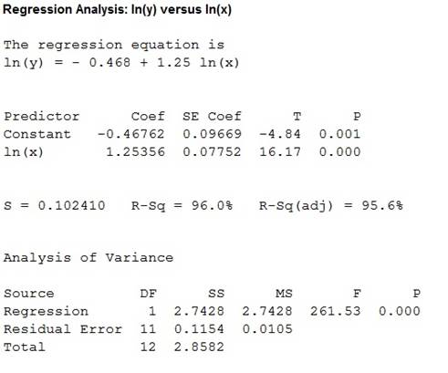
Estimate the parameters of power model.
Answer to Problem 17E
The estimate the parameters of power model are 0.626 and 1.254x.
Explanation of Solution
Given info:
The data shows the mass rate of burning x and the length of flame y.
Calculation:
The power model is given below:
Where, y is transformed into ln(y), x is transformed into ln(x).
The linear function is
The estimates of the parameters
Where,
The table below shows the calculation of estimating the parameters:
| S. No | ln(y) | ln(x) | |||
| 1 | 0.2624 | 0.5307 | 0.139256 | 0.068854 | 0.281642 |
| 2 | 0.5878 | 0.7885 | 0.46348 | 0.345509 | 0.621732 |
| 3 | 0.4701 | 0.833 | 0.391593 | 0.220994 | 0.693889 |
| 4 | 0.6932 | 0.9556 | 0.662422 | 0.480526 | 0.913171 |
| 5 | 0.742 | 0.9933 | 0.737029 | 0.550564 | 0.986645 |
| 6 | 0.7885 | 1.0987 | 0.866325 | 0.621732 | 1.207142 |
| 7 | 1.0987 | 1.1632 | 1.278008 | 1.207142 | 1.353034 |
| 8 | 0.9556 | 1.194 | 1.140986 | 0.913171 | 1.425636 |
| 9 | 1.411 | 1.411 | 1.990921 | 1.990921 | 1.990921 |
| 10 | 1.3084 | 1.4587 | 1.908563 | 1.711911 | 2.127806 |
| 11 | 1.6095 | 1.5261 | 2.456258 | 2.59049 | 2.328981 |
| 12 | 1.7579 | 1.7405 | 3.059625 | 3.090212 | 3.02934 |
| 13 | 1.6678 | 1.8083 | 3.015883 | 2.781557 | 3.269949 |
| Total | 13.3529 | 15.5016 | 18.11035 | 16.57358 | 20.22989 |
=1.253
= –0.467
Thus, the estimates of the parameters are given below:
Similarly,
b.
Construct a diagnostic plot for checking the appropriate of power model.
Answer to Problem 17E
The diagnostic plot is given below:
Explanation of Solution
Calculation:
Software procedure:
Step-by-step procedure to construct a diagnostic plot is given below:
- Choose Stats>Regression> Regression.
- Select Simple and click OK
- Under Response, choose the column containing ln(y).
- Under Predictors, choose the column containing ln(x).
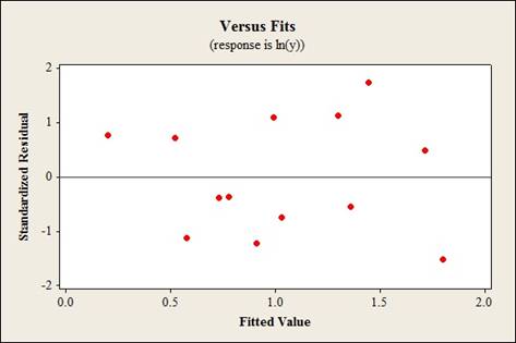
- Click Graphs, select residuals versus fits.
- Click OK.
Output obtained from MINITAB is given below:
The residual plot versus fitted values shows that the errors are randomly distributed with mean 0. This tells that the power model is appropriate to use for the given data.
The R-square value is 96% which tells that ln of mass rate of burning x can explain 96% of the variation in ln of flame length.
Hence, a power model is appropriate.
c.
Test the hypotheses
Answer to Problem 17E
There is sufficient evidence to conclude that
Explanation of Solution
Calculation:
That is, the slope coefficient equals to
That is, the slope coefficient is lesser than
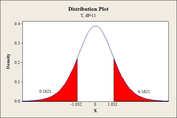
Test statistic:
=–1.032
P-value:
Software procedure:
Step-by-step procedure to find the P-value is given below:
- Choose Graph>Probability distribution Plot>View Probability.
- Select t, enter 11 for degrees of freedom.
- Under Shaded Area tab, select X value and click on Both tails.
- Enter 1.032 for X value.
- Click OK.
Output obtained from MINITAB is given below:
Conclusion:
The P-value is 0.1621 and the level of significance is 0.05.
The P-value is greater than the level of significance is 0.05.
That is, 0.1621>0.05.
Thus, the null hypothesis is not rejected.
Thus, there is sufficient evidence to conclude that
d.
Test the hypothesis that the whether the median flame with 5.0 burning rate is twice the median flame length when the burning rate is 2.5 or not.
Answer to Problem 17E
There is no sufficient evidence to conclude the median flame with 5.0 burning rate is twice the median flame length when the burning rate is 2.5
Explanation of Solution
Calculation:
The median flame with 5.0 burning rate is twice the median flame length when the burning rate is 2.5 can be expressed as,
The hypothesis test is given below:
Test statistic:
=3.265
P-value:
Software procedure:
Step-by-step procedure to find the P-value is given below:
- Choose Graph>Probability distribution Plot>View Probability.
- Select t, enter 11 for degrees of freedom.
- Under Shaded Area tab, select X value and click on Both tails.
- Enter 3.26 for X value.
- Click OK.
Output obtained from MINITAB is given below:
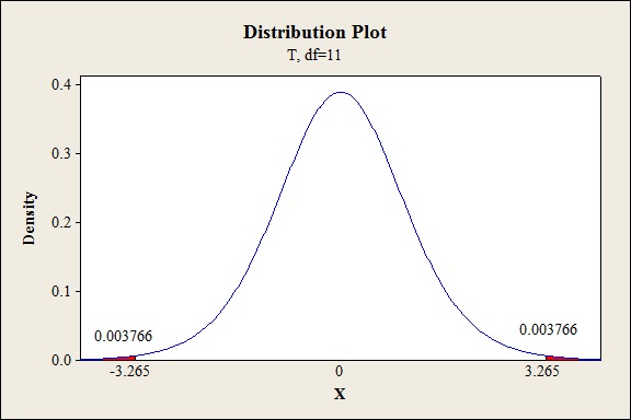
Thus, the P-value is
Conclusion:
The P-value is 0.008 and the level of significance is 0.01.
The P-value is lesser than the level of significance.
That is 0.008<0.01.
Thus, the null hypothesis is rejected.
Thus, there is no sufficient evidence to conclude the median flame with 5.0 burning rate is twice the median flame length when the burning rate is 2.5.
Want to see more full solutions like this?
Chapter 13 Solutions
Probability and Statistics for Engineering and the Sciences


- A stamped sheet steel plate is shown in Figure 164. Compute dimensions AF to 3 decimal places. All dimensions are in inches. A=_B=_C=_D=_E=_F=_arrow_forwardThe following data refers to yield of tomatoes (kg/plot) for four different levels of salinity. Salinity level here refers to electrical conductivity (EC), where the chosen levels were EC = 1.6, 3.8, 6.0, and 10.2 nmhos/cm. (Use i = 1, 2, 3, and 4 respectively.) 1.6: 59.3 53.9 56.5 63.1 58.6 3.8: 55.4 59.9 52.2 54.6 6.0: 51.2 48.3 53.1 48.9 10.2: 44.7 48.2 41.1 47.1 46.9 Use the F test at level a = 0.05 to test for any differences in true average yield due to the different salinity levels. State the appropriate hypotheses. Hạ: at least two us are equal O Ho: H = z = 43 = Ha H: all four u,'s are unequal O Ho: H = uz = H3 - Ha Hạ: at least two 4's are unequal H: all four u,'s are equal Calculate the test statistic. (Round your answer to two decimal places.)arrow_forwardThe following are the weight losses of certain machine parts due to friction (in milligrams) when used with three different lubricants: Lubricant 1: 13 11 10 13 Lubricant 2: 9. 11 Lubricant 3: 7 6. Test at the 0,01 level of significance whether the type of lubricant effects the weight loss of the machine parts due to friction. While carrying out the test, follow the steps below and answer the questions. 1- Determine the null and alternative hypotheses. Ho: H: 2-Fill in the following ANOVA Table. ANOVA Table Source of Variation Degrees of Freedom Sum of Squares Mean Sum of Squares Treatment Error Total 3-State your decision and conclusion.arrow_forward
- The following data refers to yield of tomatoes (kg/plot) for four different levels of salinity. Salinity level here refers to electrical conductivity (EC), where the chosen levels were EC = 1.6, 3.8, 6.0, and 10.2 nmhos/cm. (Use i = 1, 2, 3, and 4 respectively.) 1.6: 59.4 53.4 56.3 63.2 58.4 3.8: 55.9 59.7 52.7 54.2 6.0: 51.7 48.2 53.9 49.0 10.2: 44.3 48.3 40.7 47.2 46.7 W23 = W 24 = W34 = USE SALT Apply the modified Tukey's method to identify significant differences among us. (Round your answers to two decimal places.) W12 = W13 = W14= Which pairs are significantly different? (Select all that apply.) Othe group and the 3.8 group the 1.6 group and the 6.0 group the 1.6 group and the 10.2 group the 3.8 group and the 6.0 group the 3.8 group and the 10.2 group O the 6.0 group and the 10.2 group There are no significant differences.arrow_forwardThe following data refers to yield of tomatoes (kg/plot) for four different levels of salinity. Salinity level here refers to electrical conductivity (EC), where the chosen levels were EC = 1.6, 3.8, 6.0, and 10.2 nmhos/cm. (Use i = 1, 2, 3, and 4 respectively.) 1.6: 59.9 53.5 56.7 63.2 58.6 3.8: 55.6 59.6 52.6 54.5 6.0: 51.2 48.6 53.8 48.9 10.2: 44.3 48.4 41.0 47.9 46.5 In USE SALT Use the F test at level a = 0.05 to test for any differences in true average yield due to the different salinity levels. State the appropriate hypotheses. O Ho: H1 = H2 = !3 = H4 H: all four u's are unequal O Ho: H1 = H2 = H3 = H4 H: at least two u's are unequal O Ho: H1 # Hq # Hz# H4 H: all four u's are equal O Ho: H1* H2 * H3# H4 H: at least two u's are equal Calculate the test statistic. (Round your answer to two decimal places.) f = What can be said about the P-value for the test? O P-value > 0.100 O 0.050 < p-value < 0.100 O 0.010 < p-value < 0.050 O 0.001 < P-value < 0.010 O P-value < 0.001arrow_forwardA study of the amount of rainfall and the quantity of air pollution removed produced the following data shown in table below: Daily Rainfall x (0.01 cm) Particulate Removed y (μg/m3) 7 126 7.9 129.3 7.5 125.3 9.2 120.2 10.8 116.7 5.8 119.2 5.6 138.7 2.7 147.5 9.2 110.3 Compute and interpret the coefficient of determination, and coefficient of correlation for the given data. What will be the regression equation, when swapped depended and independent variablearrow_forward
- The data in the table below consist of measurements y₁, y2, y3, and yn of the ramus bone at four different ages on each of 20 boys. 1. Find y. 2. Find Sn 3. Find R Ramus Bone Length at Four Different Ages for 20 Boys. Age Individual 1 23 4 5 6 7 8 9 10 11 12 13 14 15 16 17 18 19 20 8 yr (yi) 47.8 46.4 46.3 45.1 47.6 52.5 51.2 49.8 48.1 45 51.2 48.5 52.1 48.2 49.6 50.7 47.2 53.3 46.2 46.3 8½ yr (Y2) 48.8 47.3 46.8 45.3 48.5 53.2 53 50 50.8 47 51.4 49.2 52.8 48.9 50.4 51.7 47.7 54.6 47.5 47.6 9 yr (Y3) 49 47.7 47.8 46.1 48.9 53.3 54.3 50.3 52.3 47.3 51.6 53 53.7 49.3 51.2 52.7 48.4 55.1 48.1 51.3 9½ yr (Y4) 49.7 48.4 48.5 47,2 49.3 53.7 54.5 52.7 54.4 48.3 51.9 55.5 55 49.8 51.8 53.3 49.5 55.3 48.4 51.8arrow_forwardAn experiment was conducted to study the extrusion process of biodegradable packaging foam. Two of the factors considered for their effect on the unit density (mg/ml) were the die temperature (145 °C vs. 155 °C) and the die diameter (3 mm vs. 4 mm). The results are stored in [Packaging Foam 1]. Source: Data extracted from W. Y. Koh, K. M. Eskridge, and M. A. Hanna, "Supersaturated Split-Plot Designs," Journal of Quality Technology, 45, January 2013, pp. 61-72.At the 0.05 level of significance, 3mm 4mm 57.22 145 72.54 145 53.60 66.70 145 48.13 49.28 145 69.89 44.14 145 62.78 58.37 145 55.18 53.98 155 57.50 63.03 155 54.17 46.73 155 73.86 60.17 155 90.28 46.78 155 88.19 43.27 155 82.61 56.93 Die Temperature a. is there an interaction between die temperature and die diameter? b. is there an effect due to die temperature? c. is there an effect due to die diameter? d. Plot the mean unit density for each die temperature for each die diameter. e. What can you conclude about the effect of die…arrow_forward10. 18.30 Temperatures are measured at various points on a heated plate (Table P18.30). Estimate the temperature at (a) x = 4, y = 3.2, and (b) x = 4.3, y = 2.7. TABLE P18.30 Temperature (°C) at various points on a square heated plate. x = 0 x = 2 y = 0 y 2 y = 4 y=6 y 8 100.00 85.00 70.00 55.00 40.00 90.00 64.49 48.90 38.78 35.00 x = 6 70.00 48.15 35.03 30.39 27.07 30.00 25.00 x = 4 80.00 53.50 38.43 x = 8 60.00 50.00 40.00 30.00 20.00arrow_forward
- In your Capstone software create a table with the following variables: Position x, m: 1, 2, 3, 4 Coefficient of friction μ: 0.36 Velocity v, m/s: v=V 2. u.9.8.xarrow_forwardThe following data represent the results obtained from the specific gravity (S.G.) test performed in a soil laboratory including for sand * ?samples. Find the modearrow_forwardThe following data are given for a biogas digester suitable for the output of six cows. The volume of digester is 8.4 m, the volume of gas holder is 2.3 m and the retention time is 26 days. Find the height of gas holder height of gas holder = cmarrow_forward
 Algebra & Trigonometry with Analytic GeometryAlgebraISBN:9781133382119Author:SwokowskiPublisher:Cengage
 Mathematics For Machine TechnologyAdvanced MathISBN:9781337798310Author:Peterson, John.Publisher:Cengage Learning,
 Calculus For The Life SciencesCalculusISBN:9780321964038Author:GREENWELL, Raymond N., RITCHEY, Nathan P., Lial, Margaret L.Publisher:Pearson Addison Wesley,
 Algebra: Structure And Method, Book 1AlgebraISBN:9780395977224Author:Richard G. Brown, Mary P. Dolciani, Robert H. Sorgenfrey, William L. ColePublisher:McDougal Littell