
Videos
The article “Effect of Environmental Factors on Steel Plate Corrosion Under Marine Immersion Conditions” (C. Soares, Y. Garbatov, and A. Zayed, Corrosion Engineering, Science and Technology, 2011:524–541) describes an experiment in which nine steel specimens were submerged in seawater at various temperatures, and the corrosion rates were measured. The results are presented in the following table (obtained by digitizing a graph).
| Temperature (°C) | Corrosion (mm/yr) |
| 26.6 | 1.58 |
| 26.0 | 1.45 |
| 27.4 | 1.13 |
| 21.7 | 0.96 |
| 14.9 | 0.99 |
| 11.3 | 1.05 |
| 15.0 | 0.82 |
| 8.7 | 0.68 |
| 8.2 | 0.56 |
- a. Construct a
scatterplot of corrosion (y) versus temperature (x). Verify that a linear model is appropriate. - b. Compute the least-squares line for predicting corrosion from temperature.
- c. Two steel specimens whose temperatures differ by 10°C are submerged in seawater. By how much would you predict their corrosion rates to differ?
- d. Predict the corrosion rate for steel submerged in seawater at a temperature of 20°C.
- e. Compute the fitted values.
- f. Compute the residuals. Which point has the residual with the largest magnitude?
- g. Compute the
correlation between temperature and corrosion rate. - h. Compute the regression sum of squares, the error sum of squares, and the total sum of squares.
- i. Divide the regression sum of squares by the total sum of squares. What is the relationship between this quantity and the
correlation coefficient ?
a.
Construct a scatterplot of corrosion (y) versus temperature (x) and also check whether the linear model is appropriate or not.
Answer to Problem 10E
The linear model is appropriate.
Explanation of Solution
Calculation:
The given information is that the data shows the temperature (°C) and corrosion (mm/yr) for 9 steel specimens.
Software Procedure:
Step-by-step procedure to obtain the scatterplot using the MINITAB software:
- Choose Graph > Scatter plot.
- Choose Simple, and then click OK.
- Under Y variables, select Corrosion.
- Under X variables, select Temperature.
- Click OK.
Output using the MINITAB software is given below:
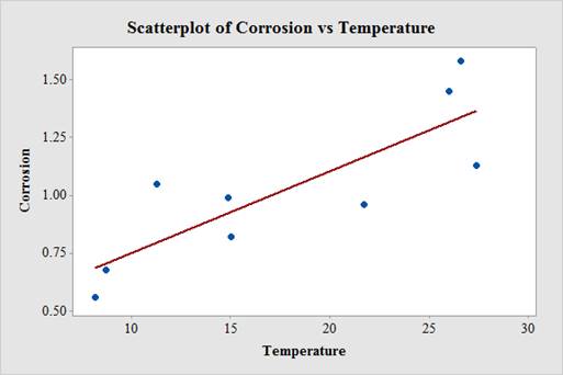
From the plot, it can be observed that the relationship between temperature and corrosion is linear. Therefore, the linear model is appropriate.
b.
Find the least-squares line for predicting corrosion from temperature.
Answer to Problem 10E
The least-squares line for predicting corrosion from temperature is
Explanation of Solution
Calculation:
Software Procedure:
Step-by-step procedure to obtain the least-squares line using the MINITAB software is given below:
- Choose Stat > Regression > Regression > Fit Regression Model.
- In Responses, enter “Corrosion”.
- In Continuous predictors, enter “Temperature”.
- Check Results.
- In Display of results, choose Simple tables.
- Click OK.
Output using the MINITAB software is given below:
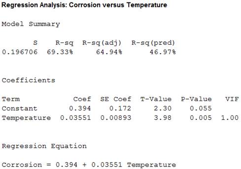
From the MINITAB output, the least-squares line for predicting corrosion from temperature is
c.
By how much would predict corrosion rates of two steel specimens to differ whose temperatures differ by 10ºC.
Explanation of Solution
Calculation:
From the least square line, the slope
The change in the predicted corrosion rates when two steel specimens whose temperatures differ by 10ºC is
Thus, the predicted corrosion rate is 0.3351 mm/yr.
d.
Predict the corrosion rate for steel submerged in seawater at a temperature of 20ºC.
Answer to Problem 10E
The predicted corrosion rate for steel submerged in seawater at a temperature of 20ºC is 1.10414 mm/yr.
Explanation of Solution
Calculation:
Predicted value:
Software Procedure:
Step-by-step procedure to obtain the predicted value using the MINITAB software:
- Stat > Regression > Regression > Predict.
- In Responses, enter “Corrosion”.
- Choose Enter individual values.
- In Temperature, enter 20.
- Click OK.
Output using the MINITAB software is given below:
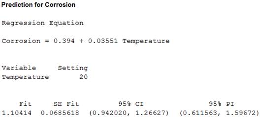
From the MINITAB output, the predicted corrosion rate for steel submerged in seawater at a temperature of 20ºC is 1.10414 mm/yr.
e.
Find the fitted values.
Answer to Problem 10E
The fitted values are, 1.33850, 1.31720, 1.36691, 1.16451, 0.92305, 0.79521, 0.92660, 0.70289 and 0.68513.
Explanation of Solution
Calculation:
Fitted value:
Software Procedure:
Step-by-step procedure to obtain the fitted value using the MINITAB software is given below:
- Choose Stat > Regression > Regression > Fit Regression Model.
- In Responses, enter “Corrosion”.
- In Continuous predictors, enter “Temperature”.
- Check Results.
- In Display of results, choose Simple tables.
- In Storage, select fits.
- Click OK.
Data display:
- Choose Data > Display data.
- In Columns, constants, and matrices to display, select FITS 1.
Output using the MINITAB software is given below:

The fitted values are, 1.33850, 1.31720, 1.36691, 1.16451, 0.92305, 0.79521, 0.92660, 0.70289 and 0.68513.
f.
Find the residuals and identify the point whose residual has the largest magnitude.
Answer to Problem 10E
The residual points are 0.241497, 0.132802, –0.236911, –0.204508, 0.066954,0.254787, –0.106597, –0.022889 and –0.125135.
The point whose residual has the largest magnitude is (11.3, 1.05).
Explanation of Solution
Calculation:
Residuals:
Software Procedure:
Step-by-step procedure to obtain the fitted value using the MINITAB software is given below:
- Choose Stat > Regression > Regression > Fit Regression Model.
- In Responses, enter “Corrosion”.
- In Continuous predictors, enter “Temperature”.
- Check Results.
- In Display of results, choose Simple tables.
- In Storage, select residuals.
- Click OK.
Data display:
- Choose Data > Display data.
- In Columns, constants, and matrices to display, select RESI 1.
Output using the MINITAB software is given below:
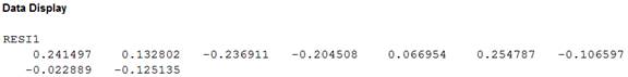
The residual points are 0.241497, 0.132802, –0.236911, –0.204508, 0.066954, 0.254787, –0.106597, –0.022889 and –0.125135.
Therefore, the point whose residual has the largest magnitude is (11.3, 1.05) because this point has the largest residual.
g.
Find the correlation between temperature and corrosion rate.
Answer to Problem 10E
The correlation between temperature and corrosion rate is 0.833.
Explanation of Solution
Calculation:
Correlation:
Software Procedure:
Step-by-step procedure to obtain the correlation using the MINITAB software:
- Select Stat > Basic Statistics > Correlation.
- In Variables, select Temperature and corrosion rate.
- Click OK.
Output using the MINITAB software is given below:
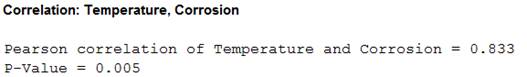
Thus, the correlation between temperature and corrosion rate is 0.833.
h.
Find the regression sum of squares, the error sum of squares, and the total sum of squares.
Answer to Problem 10E
The regression sum of squares is 0.6122, the error sum of squares is 0.2709 and the total sum of squares is 0.8830.
Explanation of Solution
Calculation:
Step-by-step procedure to obtain the regression sum of squares, the error sum of squares, and the total sum of squares using the MINITAB software is given below:
- Choose Stat > Regression > Regression > Fit Regression Model.
- In Responses, enter “Corrosion”.
- In Continuous predictors, enter “Temperature”.
- Check Results.
- In Display of results, choose Simple tables.
- Click OK.
Output using the MINITAB software is given below:
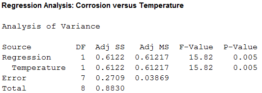
From the output, the regression sum of squares is 0.6122, the error sum of squares is 0.2709 and the total sum of squares is 0.8830.
i.
Identify the relationship between the quantity
Answer to Problem 10E
The quantity
Explanation of Solution
Calculation:
The regression sum of squares divided by the total sum of squares is
This value almost closer to the
The relationship between the quantity
Thus, the quantity
Want to see more full solutions like this?
Chapter 7 Solutions
Statistics for Engineers and Scientists
Additional Math Textbook Solutions
Business Analytics
Elementary Statistics: A Step By Step Approach
Introduction to Statistical Quality Control
Statistics for Psychology
Developmental Mathematics (9th Edition)


- An article in the Journal of Environmental Engineering (1989, Vol. 115(3), pp. 608–619) reported the results of a study on the occurrence of sodium and chloride in surface streams in central Rhode Island. The following data are chloride concentration y (in milligrams per liter) and roadway area in the watershed x (in percentage).arrow_forwardThe article “Effect of Varying Solids Concentration and Organic Loading on the Performance of Temperature Phased Anaerobic Digestion Process” (S. Vandenburgh and T. Ellis, Water Environment Research, 2002:142–148) discusses experiments to determine the effect of the solids concentration on the performance of treatment methods for wastewater sludge. In the first experiment, the concentration of solids (in g/L) was 43.94 ± 1.18. In the second experiment, which was independent of the first, the concentration was 48.66 ± 1.76. Estimate the difference in the concentration between the two experiments, and find the uncertainty in the estimate.arrow_forwardA study was conducted to compare three methods of measuring concentration of certain type of chemical pollutants in a lake. The data is given in Table 1 below. Compute SS(between) and SS(within). Compute SS(total), and explain the relationship between SS(between), SS(within), and SS(total). Compute MS(between), MS(within), and F statistic. Based on your computations, are there significant differences in the mean pollutant concentrations among the three methods? Table 1. Amount of concentration of a chemical pollutant in a lake using three different measuring methods Method 1 Method 2 Method 3 10.96 10.88 10.73 10.77 10.75 10.79 10.90 10.80 10.78 10.69 10.81 10.82 10.87 10.70 10.88 10.6 10.82 10.81 Monoamine oxidase (MAO) is an enzyme that is thought to play a role in the regulation of behavior. To see whether different categories of patients with schizophrenia have different levels of MAO activity, researchers collected…arrow_forward
- The article "Effect of Environmental Factors on Steel Plate CoIrosion Under Marine Immersion Conditions" (C. Soares, Y. Garbatov, and A. Zayed, Corrosion Engineering, Science and Technology, 2011:524-541) descrībes an experiment in which nine steel specimens were submerged in seawater at various temperatures, and the corrosion rates were measured. The results are presented in the following table (obtained by digitizing a graph). Temperature (*C) Corrosion (mnm/yr) 26.6 1.58 26.0 1.45 27.4 1.13 21.7 0.96 14.9 0.99 11.3 1.05 15.0 0.82 8.7 0.68 8.2 0.56 Construct a scatterplot of corosion (y) versus temperature (x). Verify that a linear model is appropriate. Compute the least-squares line for predicting corrosion from temperature. Two steel specimens whose temperatures differ by 10°C are submerged in seawater. By how much would you predict their corrosion rates to differ? Predict the corrosion rate for steel submerged in seawater at a temperature of 20°C. Compute the fitted values.…arrow_forwardThe article "Oxidation State and Activities of Chromium Oxides in Cao-SiO,-CrO, Slag System" (Y. Xiao, L. Holappa, and M. Reuter, Metallurgical and Materials Transactions B, 2002:595-603) presents the amount x (in mole percent) and activity coefficient y of CrO,5 for several specimens. The data, extracted from a larger table, are presented in the following table. х У 2.6 10.20 5.03 19.9 8.84 0.8 6.62 5.3 2.89 20.3 2.31 39.4 7.13 5.8 3.40 29.4 5.57 2.2 7.23 5.5 2.12 33.1 1.67 44.2 5.33 13.1 16.70 0.6 9.75 2.2 2.74 16.9 2.58 35.5 1.50 48.0 Compute the least-squares line for predicting y from x. b. Plot the residuals versus the fitted values. Compute the least-squares line for predicting y from 1/x. d. Plot the residuals versus the fitted values. C. Using the better fitting line, find a 95% confidence interval for the mean value of y when x= 5.0.arrow_forwardA study was conducted to compare three methods of measuring concentration of certain type of chemical pollutants in a lake. The data is given in Table 1 below. Compute SS(between) and SS(within). Compute SS(total), and explain the relationship between SS(between), SS(within), and SS(total). Compute MS(between), MS(within), and F statistic. Based on your computations, are there significant differences in the mean pollutant concentrations among the three methods?Table 1. Amount of concentration of a chemical pollutant in a lake using three different measuring methods Method 1 Method 2 Method 3 10.96 10.88 10.73 10.77 10.75 10.79 10.90 10.80 10.78 10.69 10.81 10.82 10.87 10.70 10.88 10.6 10.82 10.81arrow_forward
- The depth of wetting of a soil is the depth to which water content will increase owing to extemal factors. The article "Discussion of Method for Evaluation of Depth of Wetting in Residential Areas" (J. Nelson, K. Chao, and D. Overton, Journal of Geotechnical and Geoenvironmental Engineering, 2011:293-296) discusses the relationship between depth of wetting beneath a structure and the age of the structure. The article presents measurements of depth of wetting, in meters, and the ages, in years, of 21 houses, as shown in the following table. Age Depth 7.6 4 4.6 6.1 9.1 3 4.3 7.3 5.2 10.4 15.5 5.8 10.7 4 5.5 6.1 10.7 10.4 4.6 7.0 6.1 14 16.8 10 9.1 8.8 Compute the least-squares line for predicting depth of wetting (y) from age (x). b. Identify a point with an unusually large x-value. Compute the least-squares line that results from deletion of this point. Identify another point which can be classified as an outlier. Compute the least-squares line that results from deletion of the outlier,…arrow_forwardBody Fat. In the paper “Total Body Composition by Dual- Photon (153 Gd) Absorptiometry” (American Journal of Clinical Nutrition, Vol. 40, pp. 834–839), R. Mazess et al. studied methods for quantifying body composition. Eighteen randomly selected adults were measured for percentage of body fat, using dual-photon absorptiometry. Each adult’s age and percentage of body fat are shown on the WeissStats site. a. Decide whether finding a regression line for the data is reasonable. If so, then also do parts (b)–(d). b. Obtain the coefficient of determination. c. Determine the percentage of variation in the observed values of the response variable explained by the regression, and interpret your answer. d. State how useful the regression equation appears to be for making predictions.arrow_forwardBody Fat. In the paper “Total Body Composition by Dual- Photon (153 Gd) Absorptiometry” (American Journal of Clinical Nutrition, Vol. 40, pp. 834–839), R. Mazess et al. studied methods for quantifying body composition. Eighteen randomly selected adults were measured for percentage of body fat, using dual-photon absorptiometry. Each adult’s age and percentage of body fat are shown on the WeissStats site. a. Decide whether you can reasonably apply the regression t-test. If so, then also do part (b). b. Decide, at the 5% significance level, whether the data provide sufficient evidence to conclude that the predictor variable is useful for predicting the response variable.arrow_forward
- An article in Environment International ["influence of Water Temperature and Shower Head Office Size on the release Radon During Showering" (1992, Vol. 18(4)] described an experiment in which the amount of radon released in showers was imvestigated. Radon-enriched water was used in the experiment, and six different orifice diameters were tested in shower heads. The data from the experiment are shown in the following table. 5. Orifice Diameter 0.37 0.51 0.71 1.02 Radon Released () 83 75 73 72 83 85 79 79 74 76 77 67 74 74 1.40 62 62 67 69 1.99 60 64 66 (a) Does the size of the orifice affect the mean percentage of radon released? Use a=0.05. (b) Find a 95% confidence interval on the mean percent of radon released when the orifice diameter is 1.40.arrow_forwardIn the article “Groundwater Electromagnetic Imaging in Complex Geological and Topographical Regions: A Case Study of a Tectonic Boundary in the French Alps” (S. Houtot, P. Tarits, et al., Geophysics, 2002:1048–1060), the pH was measured for several water samples in various locations near Gittaz Lake in the French Alps. The results for 11 locations on the northern side of the lake and for 6 locations on the southern side are as follows: Northern side: 8.1 8.2 8.1 8.2 8.2 7.4 7.3 7.4 8.1 8.1 7.9 Southern side: 7.8 8.2 7.9 7.9 8.1 8.1 Find a 98% confidence interval for the difference in pH between the northern and southern side.arrow_forward5.25. Representative data on x = carbonation depth (in millimeters) and y = strength (in megapascals) for a sample of concrete core specimens taken from a particular building were read from a plot in the article “The Carbonation of Concrete Structures in the Tropical Environment of Singapore” (Magazine of Concrete Research [1996]: 293-300): Depth, x 8.0 20.0 20.0 30.0 35.0 40.0 50.0 55.0 65.0 Strength, y 22.8 17.1 21.1 16.1 13.4 12.4 11.4 9.7 6.8 a. Construct a scatterplot. Does the relationship between carbonation depth and strength appear to be linear? Yes, the relationship between carbonation depth and strength appears to be linear however it is a negative linear relation. b. Find the equation of the of the least-squares line.c. What would you predict for strength when carbonation depth is 25 mm?d. Explain why it would not be reasonable to use the least-squares line to predict strength when carbonation depth…arrow_forward
 MATLAB: An Introduction with ApplicationsStatisticsISBN:9781119256830Author:Amos GilatPublisher:John Wiley & Sons Inc
 Probability and Statistics for Engineering and th...StatisticsISBN:9781305251809Author:Jay L. DevorePublisher:Cengage Learning
 Statistics for The Behavioral Sciences (MindTap C...StatisticsISBN:9781305504912Author:Frederick J Gravetter, Larry B. WallnauPublisher:Cengage Learning
 Elementary Statistics: Picturing the World (7th E...StatisticsISBN:9780134683416Author:Ron Larson, Betsy FarberPublisher:PEARSON
 The Basic Practice of StatisticsStatisticsISBN:9781319042578Author:David S. Moore, William I. Notz, Michael A. FlignerPublisher:W. H. Freeman
 Introduction to the Practice of StatisticsStatisticsISBN:9781319013387Author:David S. Moore, George P. McCabe, Bruce A. CraigPublisher:W. H. Freeman