Chapter 6, Problem 1P

The tip of a one-link robot is located at $\theta =0$ at time $t=0$ s as shown in Fig. P6.1.It takes 1 for the robot to move from $\theta =0$ ,to $\theta =2\pi \text{rad}$ If $l=5$ in., plot the $x-$ and $y-$ components as a function of the. Also find the amplitude, frequency, period, phase angle, and time shift.

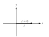
FIGURE P6.1 Rotating one-link robot starting at $\theta =0°$.

To determine

To plot:

The $x$ -component and $y$ -component as a function of time and determine the amplitude, frequency, period, phase angle and time shift.

Answer to Problem 1P

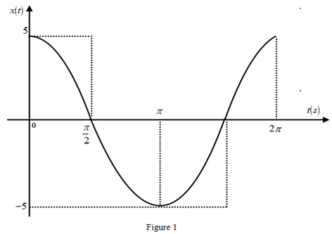
The graph for $x$ -componentas a function of timeis plotted is as shown in Figure 1.

The graph for $y$ -component as a function of time is plotted is as shown in Figure 2.

The amplitude of sine and cosine function is $5$, the frequency is $1\text{ Hz}$, the period of the tip of a one-link robot is $1\text{ s}$, the phase angle is $0\text{ rad}$ and the time shift of the one-link robot is $0\text{ s}$.

Explanation of Solution

Given:

The tip of a one-link robot is initially located at $\theta =0$ attime $t=0\text{ s}$. The given figure is shown below,

Time taken for the robot to move form $\theta =0$ to $\theta =2\pi \text{ rad}$ is $1\text{ s}$.

A one-link robot is length of $5\text{ in}$.

Concept used:

Write the expression for the linear frequency.

  $f=\frac{1}{T}$ ....... (1)

Here, $f$ is the linear frequency and $T$ is the time period.

Write the expression for the angular frequency.

  $\omega =\frac{2\pi }{T}$ ....... (2)

Here, $\omega$ is the angular frequency.

Write the expression for the time period.

  $T=\frac{2\pi }{\omega }$ ....... (3)

Write the expression for $x$ -component at any time,

  $x\left(t\right)=l\cos \left(\theta \right)$ ....... (4)

Here, $x\left(t\right)$ is the expression for $x$ -component at any time, $l$ is the length of one-link robot, $\theta$ is the angle.

Write the expression for $x$ -component at any time.

  $y\left(t\right)=l\sin \left(\theta \right)$ ....... (5)

Here, $y\left(t\right)$ is the expression for $y$ -component at any time.

Write the expression for the time shift.

  $t_0\text{=}\frac{\varphi }{\omega }$ ....... (6)

Here, $t_0$ is the expression for the time shift.

Calculation:

The one-link robot completes one revolution in $1\text{ s}$.

Substitute $1\text{ s}$ for $T$ in equation (2).

  $\begin{array}{c}\omega =\frac{2\pi }{1\text{ s}}\\ =2\pi \text{ rad/s}\end{array}$

Substitute $2\pi \text{ rad/s}$ for $\omega$ in equation (3).

  $\begin{array}{c}T=\frac{2\pi }{2\pi }\text{ s}\\ =\text{1 s}\end{array}$

Therefore, the period of the tip of a one-link robot is $1\text{ s}$.

Substitute $1\text{ s}$ for $T$ in equation (1).

  $\begin{array}{c}f=\frac{1}{1\text{ s}}\\ =1\text{ Hz}\end{array}$

Therefore, the frequency is $1\text{ Hz}$.

Since the one-link robot initially start form $\theta =0$ and the phase angle is $0\text{ rad}$.

Substitute $\omega t+\varphi$ for $\theta$ in equation (4).

  $x\left(t\right)=l\cos \left(\omega t+\varphi \right)$ ....... (7)

Here, $t$ is any given time and $\varphi$ is the phase angle.

Substitute $5\text{ in}$ for $l$, $0\text{ rad}$ for $\varphi$ and $2\pi \text{ rad/s}$ for $\omega$ in equation (7).

  $\begin{array}{c}x\left(t\right)=\left(5\right)\cos \left(\left(2\pi \right)t+0\right)\\ =5\cos 2\pi t\end{array}$

The plot for the $x$ -component as a function of time is shown in Figure 1.

Substitute $\omega t+\varphi$ for $\theta$ in equation (5).

  $y\left(t\right)=l\sin \left(\omega t+\varphi \right)$ ....... (8)

Substitute $5\text{ in}$ for $l$, $0\text{ rad}$ for $\varphi$ and $2\pi \text{ rad/s}$ for $\omega$ in equation (8).

  $\begin{array}{c}x\left(t\right)=\left(5\right)\sin \left(\left(2\pi \right)t+0\right)\\ =5\sin \left(2\pi t+0\right)\\ =5\sin \left(2\pi t\right)\end{array}$

The plot for the $y$ -component as a function of time is shown in Figure 2.

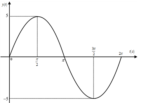
Figure 2

Substitute $0\text{ rad}$ for $\varphi$ and $2\pi \text{ rad/s}$ for $\omega$ in equation (6).

  $\begin{array}{c}{t}_0\text{ =}\frac{0\text{ rad}}{2\pi \text{ rad/s}}\\ =0\text{ s}\end{array}$

Therefore, the time shift of the one-link robot is $0\text{ s}$.

The amplitude of sine and cosine function is $5$.

Conclusion:

Thus, the graph for $x$ -component is plotted in Figure 1 and $y$ -component as a function of time is plotted in Figure 2. The amplitude of sine and cosine function is 5, the frequency is $1\text{ Hz}$, the period of the tip of a one-link robot is $1\text{ s}$, the phase angle is $0\text{ rad}$ and the time shift of the one-link robot is $0\text{ s}$.