
Videos
For the
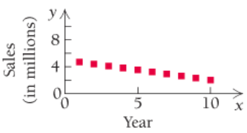
Linear,
Quadratic,
Quadratic
Polynomial, neither quadratic nor linear
Exponential,
Want to see the full answer?
Check out a sample textbook solution
Chapter R Solutions
Calculus and Its Applications (11th Edition)
Additional Math Textbook Solutions
Single Variable Calculus: Early Transcendentals (2nd Edition) - Standalone book
Precalculus: Concepts Through Functions, A Unit Circle Approach to Trigonometry (4th Edition)
Calculus & Its Applications (14th Edition)
Thomas' Calculus: Early Transcendentals (14th Edition)
Calculus: Early Transcendentals (3rd Edition)
University Calculus: Early Transcendentals (4th Edition)


- The following table gives the millions of metric tons of carbon dioxide emissions in a certain country for selected years from 2010 and projected to 2032. Year 2010 2012 2014 2016 2018 2020 CO2 Emissions 337.5 361.5 395.1 425.8 451.1 496.4 Year 2022 2024 2026 2028 2030 2032 CO2 Emissions 558.2 592.9 628.7 662.1 709.1 742.7 (a) Create a linear function that models these data, with x as the number of years past 2010 and y as the millions of metric tons of carbon dioxide emissions. (Round all numerical values to two decimal places.)y(x) = (b) Find the model's estimate for the 2028 data point. (Round your answer to two decimal places.) million metric tons(c) Find the slope of the linear model. (Round your answer to two decimal places.)Interpret the slope of the linear model. For each year since ---Select--- 2009 2010 2015 2028 2032 , carbon dioxide emissions in the U.S. are expected to change by million metric tons.arrow_forwardfind the linearization at x = a. y = e√x , a = 1arrow_forwardThe following table shows students’ test scores on the first two tests in an introductory statistics class. Statistics Test Scores First test, x 7575 7676 9191 6565 4848 7575 8585 6262 5151 8080 9494 4343 Second test, y 6969 8888 101101 6363 5959 8282 8686 6767 5656 8484 105105 4444 Copy Data Step 1 of 2 : Find an equation of the least-squares regression line. Round your answer to three decimal places, if necessary.arrow_forward
- Find the linearization L(x)of the function at a .arrow_forwardThe following table shows data for the cost of natural gas in Maryland (in dollars per Million Btu) for x years since 1990. Year x Price in $ per Million Btu 1990 6.31 1991 6.14 1992 6.32 1993 6.75 1994 6.8 1995 6.34 1996 7.46 1997 8.12 1998 8.04 1999 8.25 2000 9.58 2001 11.28 2002 9.25 a. Predict the price in dollars per million Btu for the year 2010. Then calculate the residual for the year 2010 if the actual price in 2010 was $11.57 per million Btu. b. What is the correlation coefficient, rounded to two decimal places. Is the linear association between the variables “weak” or “strong”? How do you know?arrow_forwardUse this data and create a model that estimates a student's giving rate as an alumni based on the three parameters provided. If a class has a graduation rate of 74, the % of classes under 20 student equal to 55, and a Student=Faculty Ratio of 19, what should we expect our Alumni Giving Rate to be? (Enter a whole number) University Graduation Rate % of Classes Under 20 Student-Faculty Ratio Alumni Giving Rate Boston College 85 39 13 25 Brandeis University 79 68 8 33 Brown University 93 60 8 40 California Institute of Technology 85 65 3 46 Carnegie Mellon University 75 67 10 28 Case Western Reserve Univ. 72 52 8 31 College of William and Mary 89 45 12 27 Columbia University 90 69 7 31 Cornell University 91 72 13 35 Dartmouth College 94 61 10 53 Duke University 92 68 8 45 Emory University 84 65 7 37 Georgetown University 91 54 10 29 Harvard University 97 73 8 46 Johns Hopkins University 89 64 9 27 Lehigh University 81 55 11 40 Massachusetts Inst.…arrow_forward
- Find the linearization L(x) of y=e10xln(x) at a=1arrow_forward2. Chapter 14 Review 45: Calculate ∂z∂x , where xez + zey = x + y.arrow_forwardThe table below contains the average public school classroom teacher's salaries, , for an 11-year period. Letting represent 1990, use a graphing utility to find a linear model for the data. Year 1990 1991 1992 1993 1994 1995 Salary 32669 33462 35288 35692 37007 36266 Year 1996 1997 1998 1999 2000 Salary 37004 40108 41236 41937 43676 Salary, written as a function of is given byarrow_forward
- Use this data and develop a model of a truck's annual maintenance expenses based on its weekly usage in hours. b1 = (Keep three decimal places) Weekly Usage (hours) Annual Maintenance Expense 13 17.0 10 22.0 14 25.0 18 27.0 22 37.0 27 34.0 25 33.0 31 39.0 40 51.5 38 40.0arrow_forwardUse this data and develop a model of a truck's annual maintenance expenses based on its weekly usage in hours. SSR = ? (Keep one decimal place) Weekly Usage (hours) Annual Maintenance Expense 13 17.0 10 22.0 20 30.0 28 37.0 32 47.0 17 30.5 24 32.5 31 39.0 40 51.5 38 40.0arrow_forwardIn Exercises 9-20, use the Chain Rule to calculate - f(r(t)) at the value dt of t given.arrow_forward
 Algebra & Trigonometry with Analytic GeometryAlgebraISBN:9781133382119Author:SwokowskiPublisher:Cengage
 Big Ideas Math A Bridge To Success Algebra 1: Stu...AlgebraISBN:9781680331141Author:HOUGHTON MIFFLIN HARCOURTPublisher:Houghton Mifflin Harcourt