
Videos
The accompanying summary data on compression strength (lb) for 12 × 10 × 8 in. boxes appeared in the article “Compression of Single-Wall Corrugated Shipping Containers Using Fixed and Floating Test Platens” (J. Testing and Evaluation, 1992: 318–320). The authors stated that “the difference between the compression strength using fixed and floating platen method was found to be small compared to normal variation in compression strength between identical boxes.” Do you agree? Is your analysis predicated on any assumptions?
| Sample | Sample | Sample | |
| Method | Size | SD | |
| Fixed | 10 | 807 | 27 |
| Floating | 10 | 757 | 41 |
Check whether the claim that the “difference between compression strength using fixed method and floating platen is smaller than the normal variation in compression strength between identical boxes” is appropriate.
Check whether the analysis is based on any assumptions.
Answer to Problem 67SE
The authors claim that “difference between compression strength using fixed method and floating platen is smaller than the normal variation in compression strength between identical boxes” is not agreed.
Yes, the analysis is based on certain assumptions.
Explanation of Solution
Given info:
Let
Calculation:
Here,
The test hypotheses are,
Null hypothesis:
That is, the mean compression strength fixed method is different from the floating platen method.
Alternative hypothesis:
That is, there is evidence that the mean compression strength fixed method is different from the floating platen method.
Assumption for the two sample t-test:
- The samples X and Y are selected from the population at random.
- The samples X and Y are independent of each other.
- Samples must be distributed normally.
Here, the samples selected from the fixed method and floating method were selected at random and independently. Moreover, the sample size is large and distributed normally. Hence, the assumptions are satisfied.
Conduct the two-sample t-test to test the hypotheses.
Test statistic:
Step-by-step procedure to obtain the test statistic using the MINITAB software:
- Choose Stat > Basic Statistics > 2-Sample t.
- Choose Sample from the columns.
- In first, enter Sample size as 10, Mean as 807, Standard deviation as 27.
- In second, enter Sample size as 10, Mean as 757, Standard deviation as 41.
- Choose Options.
- In Confidence level, enter 95.
- In Alternative, select Not equal.
- Click OK in all the dialog boxes.
Output using the MINITAB software is given below:
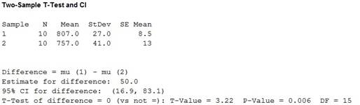
From the output, the test statistic is 3.22 and the P- value is 0.006.
Rejection rule:
If
Conclusion:
Here, the P-value is less than the level of significance.
That is,
Therefore, the decision is “reject the null hypothesis”.
Thus, it can be concluded that there is evidence that the mean compression strength fixed method is different from the floating platen method.
The authors claim that “difference between compression strength using fixed method and floating platen is smaller than the normal variation in compression strength between identical boxes” is not agreed.
Here, the sample size of the compression strength data is small and it is assumed to be distributed to normal. Also, it is assumed that the data were selected at random and independent.
Want to see more full solutions like this?
Chapter 9 Solutions
Probability and Statistics for Engineering and the Sciences


- The article “Effect of Internal Gas Pressure on the Com- pression Strength of Beverage Cans and Plastic Bottles” (J. of Testing and Evaluation, 1993: 129–131) includes the accompanying data on compression strength (lb) for a sample of 12-oz aluminum cans filled with strawberry drink and another sample filled with cola. Does the data suggest that the extra carbonation of cola results in a higher average compression strength? Base your answer on a P-value. What assumptions are necessary for your analysis? ( use ? = 0.01 )arrow_forwardThe article “Structural Performance of Rounded Dovetail Connections Under Different Loading Conditions” (T. Tannert, H. Prion, and F. Lam, Can J Civ Eng, 2007:1600–1605) describes a study of the deformation properties of dovetail joints. In one experiment, 10 rounded dovetail connections and 10 double rounded dovetail connections were loaded until failure. The rounded connections had an average load at failure of 8.27 kN with a standard deviation of 0.62 kN. The double-rounded connections had an average load at failure of 6.11 kN with a standard deviation of 1.31 kN. Can you conclude that the mean load at failure is greater for rounded connections than for double-rounded connections?arrow_forwardConsider the following summary data on the modulus of elasticity (✕ 106 psi) for lumber of three different grades. Grade J xi. si 1 9 1.61 0.21 2 9 1.55 0.25 3 9 1.44 0.23 Use this data and a significance level of 0.01 to test the null hypothesis of no difference in mean modulus of elasticity for the three grades. Calculate the test statistic. (Round your answer to two decimal places.) f = What can be said about the P-value for the test? P-value > 0.100 0.050 < P-value < 0.100 0.010 < P-value < 0.050 0.001 < P-value < 0.010 P-value < 0.001 What can you conclude? Reject H0. At least two of the three grades appear to differ significantly. Reject H0. The three grades do not appear to differ significantly. Fail to reject H0. The three grades do not appear to differ significantly. Fail to reject H0. At least two of the three grades appear to differ significantly.arrow_forward
- A law enforcement organization claims that their radargun is accurate to within 0.5 miles per hour for a courthearing. An independent organization hired to test theaccuracy of the radar gun conducted 12 tests on a projectilemoving at 60 miles per hour. Given the data inthe following table, determine if the radar gun can beused in court. State the hypothesis and base your commentson an appropriate α level.arrow_forwardThe value of Young’s modulus (GPa) was determined forcast plates consisting of certain intermetallic substrates,resulting in the following sample observations (“Strengthand Modulus of a Molybdenum-Coated Ti-25Al-10Nb-3U-1Mo Intermetallic,” J. of Materials Engr.and Performance, 1997: 46–50):116.4 115.9 114.6 115.2 115.8a. Calculate x and the deviations from the mean.b. Use the deviations calculated in part (a) to obtain thesample variance and the sample standard deviation.c. Calculate s2 by using the computational formula forthe numerator Sxx.d. Subtract 100 from each observation to obtain a sampleof transformed values. Now calculate the samplevariance of these transformed values, and compare itto s2 for the original data.arrow_forwardA researcher estimates that the average height of the buildings of 30 or more stories in a large city is at most 700 feet. A random sample of 10 buildings is selected, and the heights in feet are shown. At α = 0.025, is there enough evidence to reject the claim? 485 511 841 725 615 520 535 635 616 582 What is the critical value of the t?arrow_forward
- Two quality control technicians measured the surface finish of a metal part, obtaining the data in the table below. Assume that the measurements are normally distributed.arrow_forwardONLY THE LAST ONE Consider the accompanying data on flexural strength (MPa) for concrete beams of a certain type. 5.9 7.2 7.3 6.3 8.1 6.8 7.0 7.5 6.8 6.5 7.0 6.3 7.9 9.0 8.4 8.7 7.8 9.7 7.4 7.7 9.7 8.2 7.7 11.6 11.3 11.8 10.7 The data below give accompanying strength observations for cylinders. 6.5 5.8 7.8 7.1 7.2 9.2 6.6 8.3 7.0 8.3 7.8 8.1 7.4 8.5 8.9 9.8 9.7 14.1 12.6 11.9 Prior to obtaining data, denote the beam strengths by X1, . . . , Xm and the cylinder strengths by Y1, . . . , Yn. Suppose that the Xi's constitute a random sample from a distribution with mean μ1 and standard deviation σ1 and that the Yi's form a random sample (independent of the Xi's) from another distribution with mean μ2 and standard deviation σ2. (a) Use rules of expected value to show that X − Y is an unbiased estimator of μ1 − μ2. E(X − Y) = E(X) − E(Y) = μ1 − μ2 E(X − Y) = E(X) − E(Y) 2 = μ1 − μ2 E(X − Y) = nm E(X) − E(Y) = μ1 − μ2 E(X −…arrow_forwardA snack food manufacturer estimates that the variance of the number of grams of carbohydrates in servings of its tortilla chips is 1.34. A dietician is asked to test this claim and finds that a random sample of 16 servings has a variance of 1.22. At α=0.05, is there enough evidence to reject the manufacturer's claim? Assume the population is normally distributed. Complete parts (a) through (e) below.arrow_forward
- Consider the accompanying data on flexural strength (MPa) for concrete beams of a certain type. 8.3 7.4 7.0 6.8 7.8 9.7 5.0 6.3 6.8 9.0 7.7 7.3 7.4 11.8 6.3 7.7 11.6 7.2 11.3 9.7 10.7 7.0 7.9 8.7 7.9 8.1 6.5 (a) Calculate a point estimate of the mean value of strength for the conceptual population of all beams manufactured in this fashion. [Hint: Σxi = 218.9.] (Round your answer to three decimal places.) MPa(b) Calculate a point estimate of the strength value that separates the weakest 50% of all such beams from the strongest 50%. MPa(c) Calculate a point estimate of the population standard deviation ?. [Hint: Σxi2 = 1851.35.] (Round your answer to three decimal places.) MPa(d) Calculate a point estimate of the proportion of all such beams whose flexural strength exceeds 10 MPa. [Hint: Think of an observation as a "success" if it exceeds 10.] (Round your answer to three decimal places.)(e) Calculate a point estimate of the population coefficient of variation ?/?. (Round…arrow_forwardLactation promotes a temporary loss of bone mass to provide adequate amounts of calcium for milk production. The paper “Bone Mass Is Recovered from Lactation to Postweaning in Adolescent Mothers with Low Calcium Intakes” (Amer. J. of Clinical Nutr., 2004: 1322–1326) gave the following data on total body bone mineral content (TBBMC) (g) for a sample both during lactation (L) and in the postweaning period (P). SubjectL 1928 2549 2825 1924 1628 2175 2114 2621 1843 2541P 2126 2885 2895 1942 1750 2184 2164 2626 2006 2627 Does the data suggest that true average total body bone mineral content during postweaning exceeds that during lactation by more than 25 g? State and test the appropriate hypotheses using a significance level of .05.arrow_forwardAn experiment to determine the effect of four different types of engine oil (A, B, C, and D) on the rolling friction coefficient of a car speed has been conducted. Three brands of car (Honda, Toyota, and Mazda) were chosen, and each engine oil was tested twice on each car, producing the following ANOVA output in Figure 2. i) How many treatments involved? Write down all the treatments ii) Identify the number of replication for each treatment. iii) Based on the ANOVA table above, find the values of W, X, Y and Z. iv) Test the interaction effect on rolling friction coefficient of car speed between the four different types of engine oil and the three different brands of car. v) Do we need to test for marginal effect? Give a reason.arrow_forward
 MATLAB: An Introduction with ApplicationsStatisticsISBN:9781119256830Author:Amos GilatPublisher:John Wiley & Sons Inc
 Probability and Statistics for Engineering and th...StatisticsISBN:9781305251809Author:Jay L. DevorePublisher:Cengage Learning
 Statistics for The Behavioral Sciences (MindTap C...StatisticsISBN:9781305504912Author:Frederick J Gravetter, Larry B. WallnauPublisher:Cengage Learning
 Elementary Statistics: Picturing the World (7th E...StatisticsISBN:9780134683416Author:Ron Larson, Betsy FarberPublisher:PEARSON
 The Basic Practice of StatisticsStatisticsISBN:9781319042578Author:David S. Moore, William I. Notz, Michael A. FlignerPublisher:W. H. Freeman
 Introduction to the Practice of StatisticsStatisticsISBN:9781319013387Author:David S. Moore, George P. McCabe, Bruce A. CraigPublisher:W. H. Freeman