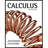
Calculus - Standalone book
3rd Edition
ISBN: 9781464125263
Author: Jon Rogawski, Colin Adams
Publisher: W.H. Freeman & Co
expand_more
expand_more
format_list_bulleted
Concept explainers
Question
Chapter 6.1, Problem 62E
To determine
Calculate the Gini index of the United States in the year
Expert Solution & Answer
Want to see the full answer?
Check out a sample textbook solution
Students have asked these similar questions
Alcohol use in the United States increased during the first year of the COVID pandemic, as did the
number of alcohol-induced deaths (such as alcoholic liver disease, accidental alcohol poisoning,
disorders due to acute intoxication).
Here is a figure from the CDC representing the "Rates of alcohol-induced deaths in the United
States in 2020, broken down by sex and age group."
Figure 2. Rates of alcohol-induced deaths, by sex and age group: United States, 2020
Age group (years)
Under 25 0.1
25-34
35-44
45-54
55-64
65-74
75-84
85 and over
Under 25
25-34
35-44
45-54
55-64
65-74
75-84
85 and over
0
0.3
3.9
2.9
6.4
10.2
7.9
10
12.9
12.8
16.7
20
21.0
21.8
24.5
Female
Male
38.5
SOURCE: National Center for Health Statistics, National Vital Statistics System, Mortality.
I
40
43.4
30
Deaths per 100,000 population
50
59.0
I
60
70
Interpret the bottom-most bar (gray bar with the value "12.8" written next to it) as a sentence in
context.
Enter your answer here
Select ALL correct interpretations of…
what is z observed?
Calculate Harmonic from the following statistical data :
Wages:
10
12
14
16
18
No. of workers:
2
5
8 3
2.
Chapter 6 Solutions
Calculus - Standalone book
Ch. 6.1 - Prob. 1PQCh. 6.1 - Prob. 2PQCh. 6.1 - Prob. 3PQCh. 6.1 - Prob. 4PQCh. 6.1 - Prob. 5PQCh. 6.1 - Prob. 6PQCh. 6.1 - Prob. 1ECh. 6.1 - Prob. 2ECh. 6.1 - Prob. 3ECh. 6.1 - Prob. 4E
Ch. 6.1 - Prob. 5ECh. 6.1 - Prob. 6ECh. 6.1 - Prob. 7ECh. 6.1 - Prob. 8ECh. 6.1 - Prob. 9ECh. 6.1 - Prob. 10ECh. 6.1 - Prob. 11ECh. 6.1 - Prob. 12ECh. 6.1 - Prob. 13ECh. 6.1 - Prob. 14ECh. 6.1 - Prob. 15ECh. 6.1 - Prob. 16ECh. 6.1 - Prob. 17ECh. 6.1 - Prob. 18ECh. 6.1 - Prob. 19ECh. 6.1 - Prob. 20ECh. 6.1 - Prob. 21ECh. 6.1 - Prob. 22ECh. 6.1 - Prob. 23ECh. 6.1 - Prob. 24ECh. 6.1 - Prob. 25ECh. 6.1 - Prob. 26ECh. 6.1 - Prob. 27ECh. 6.1 - Prob. 28ECh. 6.1 - Prob. 29ECh. 6.1 - Prob. 30ECh. 6.1 - Prob. 31ECh. 6.1 - Prob. 32ECh. 6.1 - Prob. 33ECh. 6.1 - Prob. 34ECh. 6.1 - Prob. 35ECh. 6.1 - Prob. 36ECh. 6.1 - Prob. 37ECh. 6.1 - Prob. 38ECh. 6.1 - Prob. 39ECh. 6.1 - Prob. 40ECh. 6.1 - Prob. 41ECh. 6.1 - Prob. 42ECh. 6.1 - Prob. 43ECh. 6.1 - Prob. 44ECh. 6.1 - Prob. 45ECh. 6.1 - Prob. 46ECh. 6.1 - Prob. 47ECh. 6.1 - Prob. 48ECh. 6.1 - Prob. 49ECh. 6.1 - Prob. 50ECh. 6.1 - Prob. 51ECh. 6.1 - Prob. 52ECh. 6.1 - Prob. 53ECh. 6.1 - Prob. 54ECh. 6.1 - Prob. 55ECh. 6.1 - Prob. 56ECh. 6.1 - Prob. 57ECh. 6.1 - Prob. 58ECh. 6.1 - Prob. 59ECh. 6.1 - Prob. 60ECh. 6.1 - Prob. 61ECh. 6.1 - Prob. 62ECh. 6.1 - Prob. 63ECh. 6.1 - Prob. 64ECh. 6.2 - Prob. 1PQCh. 6.2 - Prob. 2PQCh. 6.2 - Prob. 3PQCh. 6.2 - Prob. 4PQCh. 6.2 - Prob. 5PQCh. 6.2 - Prob. 1ECh. 6.2 - Prob. 2ECh. 6.2 - Prob. 3ECh. 6.2 - Prob. 4ECh. 6.2 - Prob. 5ECh. 6.2 - Prob. 6ECh. 6.2 - Prob. 7ECh. 6.2 - Prob. 8ECh. 6.2 - Prob. 9ECh. 6.2 - Prob. 10ECh. 6.2 - Prob. 11ECh. 6.2 - Prob. 12ECh. 6.2 - Prob. 13ECh. 6.2 - Prob. 14ECh. 6.2 - Prob. 15ECh. 6.2 - Prob. 16ECh. 6.2 - Prob. 17ECh. 6.2 - Prob. 18ECh. 6.2 - Prob. 19ECh. 6.2 - Prob. 20ECh. 6.2 - Prob. 21ECh. 6.2 - Prob. 22ECh. 6.2 - Prob. 23ECh. 6.2 - Prob. 24ECh. 6.2 - Prob. 25ECh. 6.2 - Prob. 26ECh. 6.2 - Prob. 27ECh. 6.2 - Prob. 28ECh. 6.2 - Prob. 29ECh. 6.2 - Prob. 30ECh. 6.2 - Prob. 31ECh. 6.2 - Prob. 32ECh. 6.2 - Prob. 33ECh. 6.2 - Prob. 34ECh. 6.2 - Prob. 35ECh. 6.2 - Prob. 36ECh. 6.2 - Prob. 37ECh. 6.2 - Prob. 38ECh. 6.2 - Prob. 39ECh. 6.2 - Prob. 40ECh. 6.2 - Prob. 41ECh. 6.2 - Prob. 42ECh. 6.2 - Prob. 43ECh. 6.2 - Prob. 44ECh. 6.2 - Prob. 45ECh. 6.2 - Prob. 46ECh. 6.2 - Prob. 47ECh. 6.2 - Prob. 48ECh. 6.2 - Prob. 49ECh. 6.2 - Prob. 50ECh. 6.2 - Prob. 51ECh. 6.2 - Prob. 52ECh. 6.2 - Prob. 53ECh. 6.2 - Prob. 54ECh. 6.2 - Prob. 55ECh. 6.2 - Prob. 56ECh. 6.2 - Prob. 57ECh. 6.2 - Prob. 58ECh. 6.2 - Prob. 59ECh. 6.2 - Prob. 60ECh. 6.2 - Prob. 61ECh. 6.2 - Prob. 62ECh. 6.2 - Prob. 63ECh. 6.2 - Prob. 64ECh. 6.2 - Prob. 65ECh. 6.2 - Prob. 66ECh. 6.2 - Prob. 67ECh. 6.2 - Prob. 68ECh. 6.3 - Prob. 1PQCh. 6.3 - Prob. 2PQCh. 6.3 - Prob. 3PQCh. 6.3 - Prob. 4PQCh. 6.3 - Prob. 1ECh. 6.3 - Prob. 2ECh. 6.3 - Prob. 3ECh. 6.3 - Prob. 4ECh. 6.3 - Prob. 5ECh. 6.3 - Prob. 6ECh. 6.3 - Prob. 7ECh. 6.3 - Prob. 8ECh. 6.3 - Prob. 9ECh. 6.3 - Prob. 10ECh. 6.3 - Prob. 11ECh. 6.3 - Prob. 12ECh. 6.3 - Prob. 13ECh. 6.3 - Prob. 14ECh. 6.3 - Prob. 15ECh. 6.3 - Prob. 16ECh. 6.3 - Prob. 17ECh. 6.3 - Prob. 18ECh. 6.3 - Prob. 19ECh. 6.3 - Prob. 20ECh. 6.3 - Prob. 21ECh. 6.3 - Prob. 22ECh. 6.3 - Prob. 23ECh. 6.3 - Prob. 24ECh. 6.3 - Prob. 25ECh. 6.3 - Prob. 26ECh. 6.3 - Prob. 27ECh. 6.3 - Prob. 28ECh. 6.3 - Prob. 29ECh. 6.3 - Prob. 30ECh. 6.3 - Prob. 31ECh. 6.3 - Prob. 32ECh. 6.3 - Prob. 33ECh. 6.3 - Prob. 34ECh. 6.3 - Prob. 35ECh. 6.3 - Prob. 36ECh. 6.3 - Prob. 37ECh. 6.3 - Prob. 38ECh. 6.3 - Prob. 39ECh. 6.3 - Prob. 40ECh. 6.3 - Prob. 41ECh. 6.3 - Prob. 42ECh. 6.3 - Prob. 43ECh. 6.3 - Prob. 44ECh. 6.3 - Prob. 45ECh. 6.3 - Prob. 46ECh. 6.3 - Prob. 47ECh. 6.3 - Prob. 48ECh. 6.3 - Prob. 49ECh. 6.3 - Prob. 50ECh. 6.3 - Prob. 51ECh. 6.3 - Prob. 52ECh. 6.3 - Prob. 53ECh. 6.3 - Prob. 54ECh. 6.3 - Prob. 55ECh. 6.3 - Prob. 56ECh. 6.3 - Prob. 57ECh. 6.3 - Prob. 58ECh. 6.3 - Prob. 59ECh. 6.3 - Prob. 60ECh. 6.3 - Prob. 61ECh. 6.3 - Prob. 62ECh. 6.3 - Prob. 63ECh. 6.3 - Prob. 64ECh. 6.4 - Prob. 1PQCh. 6.4 - Prob. 2PQCh. 6.4 - Prob. 3PQCh. 6.4 - Prob. 1ECh. 6.4 - Prob. 2ECh. 6.4 - Prob. 3ECh. 6.4 - Prob. 4ECh. 6.4 - Prob. 5ECh. 6.4 - Prob. 6ECh. 6.4 - Prob. 7ECh. 6.4 - Prob. 8ECh. 6.4 - Prob. 9ECh. 6.4 - Prob. 10ECh. 6.4 - Prob. 11ECh. 6.4 - Prob. 12ECh. 6.4 - Prob. 13ECh. 6.4 - Prob. 15ECh. 6.4 - Prob. 16ECh. 6.4 - Prob. 17ECh. 6.4 - Prob. 18ECh. 6.4 - Prob. 19ECh. 6.4 - Prob. 20ECh. 6.4 - Prob. 21ECh. 6.4 - Prob. 22ECh. 6.4 - Prob. 23ECh. 6.4 - Prob. 24ECh. 6.4 - Prob. 25ECh. 6.4 - Prob. 26ECh. 6.4 - Prob. 27ECh. 6.4 - Prob. 28ECh. 6.4 - Prob. 29ECh. 6.4 - Prob. 30ECh. 6.4 - Prob. 31ECh. 6.4 - Prob. 32ECh. 6.4 - Prob. 33ECh. 6.4 - Prob. 34ECh. 6.4 - Prob. 35ECh. 6.4 - Prob. 36ECh. 6.4 - Prob. 37ECh. 6.4 - Prob. 38ECh. 6.4 - Prob. 39ECh. 6.4 - Prob. 40ECh. 6.4 - Prob. 41ECh. 6.4 - Prob. 42ECh. 6.4 - Prob. 43ECh. 6.4 - Prob. 44ECh. 6.4 - Prob. 45ECh. 6.4 - Prob. 46ECh. 6.4 - Prob. 47ECh. 6.4 - Prob. 48ECh. 6.4 - Prob. 49ECh. 6.4 - Prob. 50ECh. 6.4 - Prob. 51ECh. 6.4 - Prob. 52ECh. 6.4 - Prob. 53ECh. 6.4 - Prob. 54ECh. 6.4 - Prob. 55ECh. 6.4 - Prob. 56ECh. 6.4 - Prob. 57ECh. 6.4 - Prob. 58ECh. 6.4 - Prob. 59ECh. 6.4 - Prob. 60ECh. 6.4 - Prob. 61ECh. 6.4 - Prob. 62ECh. 6.5 - Prob. 1PQCh. 6.5 - Prob. 2PQCh. 6.5 - Prob. 3PQCh. 6.5 - Prob. 4PQCh. 6.5 - Prob. 1ECh. 6.5 - Prob. 2ECh. 6.5 - Prob. 3ECh. 6.5 - Prob. 4ECh. 6.5 - Prob. 5ECh. 6.5 - Prob. 6ECh. 6.5 - Prob. 7ECh. 6.5 - Prob. 8ECh. 6.5 - Prob. 9ECh. 6.5 - Prob. 10ECh. 6.5 - Prob. 11ECh. 6.5 - Prob. 12ECh. 6.5 - Prob. 13ECh. 6.5 - Prob. 14ECh. 6.5 - Prob. 15ECh. 6.5 - Prob. 16ECh. 6.5 - Prob. 17ECh. 6.5 - Prob. 18ECh. 6.5 - Prob. 19ECh. 6.5 - Prob. 20ECh. 6.5 - Prob. 21ECh. 6.5 - Prob. 22ECh. 6.5 - Prob. 23ECh. 6.5 - Prob. 24ECh. 6.5 - Prob. 25ECh. 6.5 - Prob. 26ECh. 6.5 - Prob. 27ECh. 6.5 - Prob. 28ECh. 6.5 - Prob. 29ECh. 6.5 - Prob. 30ECh. 6.5 - Prob. 31ECh. 6.5 - Prob. 32ECh. 6.5 - Prob. 33ECh. 6.5 - Prob. 34ECh. 6.5 - Prob. 35ECh. 6.5 - Prob. 36ECh. 6.5 - Prob. 37ECh. 6.5 - Prob. 38ECh. 6.5 - Prob. 39ECh. 6.5 - Prob. 40ECh. 6.5 - Prob. 41ECh. 6.5 - Prob. 42ECh. 6.5 - Prob. 43ECh. 6 - Prob. 1CRECh. 6 - Prob. 2CRECh. 6 - Prob. 3CRECh. 6 - Prob. 4CRECh. 6 - Prob. 5CRECh. 6 - Prob. 6CRECh. 6 - Prob. 7CRECh. 6 - Prob. 8CRECh. 6 - Prob. 9CRECh. 6 - Prob. 10CRECh. 6 - Prob. 11CRECh. 6 - Prob. 12CRECh. 6 - Prob. 13CRECh. 6 - Prob. 14CRECh. 6 - Prob. 15CRECh. 6 - Prob. 16CRECh. 6 - Prob. 17CRECh. 6 - Prob. 18CRECh. 6 - Prob. 19CRECh. 6 - Prob. 20CRECh. 6 - Prob. 21CRECh. 6 - Prob. 22CRECh. 6 - Prob. 23CRECh. 6 - Prob. 24CRECh. 6 - Prob. 25CRECh. 6 - Prob. 26CRECh. 6 - Prob. 27CRECh. 6 - Prob. 28CRECh. 6 - Prob. 29CRECh. 6 - Prob. 30CRECh. 6 - Prob. 31CRECh. 6 - Prob. 32CRECh. 6 - Prob. 33CRECh. 6 - Prob. 34CRECh. 6 - Prob. 35CRECh. 6 - Prob. 36CRECh. 6 - Prob. 37CRECh. 6 - Prob. 38CRECh. 6 - Prob. 39CRECh. 6 - Prob. 40CRECh. 6 - Prob. 41CRECh. 6 - Prob. 42CRECh. 6 - Prob. 43CRECh. 6 - Prob. 44CRECh. 6 - Prob. 45CRECh. 6 - Prob. 46CRECh. 6 - Prob. 47CRECh. 6 - Prob. 48CRECh. 6 - Prob. 49CRECh. 6 - Prob. 50CRECh. 6 - Prob. 51CRECh. 6 - Prob. 52CRECh. 6 - Prob. 53CRECh. 6 - Prob. 54CRE
Knowledge Booster
Learn more about
Need a deep-dive on the concept behind this application? Look no further. Learn more about this topic, calculus and related others by exploring similar questions and additional content below.Similar questions
- What does the y -intercept on the graph of a logistic equation correspond to for a population modeled by that equation?arrow_forwardFind the mean hourly cost when the cell phone described above is used for 240 minutes.arrow_forwardTable 6 shows the population, in thousands, of harbor seals in the Wadden Sea over the years 1997 to 2012. a. Let x represent time in years starting with x=0 for the year 1997. Let y represent the number of seals in thousands. Use logistic regression to fit a model to these data. b. Use the model to predict the seal population for the year 2020. c. To the nearest whole number, what is the limiting value of this model?arrow_forward
- Thirty AA batteries were tested to determine how long they would last. The results, to the nearest minute, were recorded as follows: Table 3: Life of AA batteries, in minutes Battery life, x (in minutes) Number of battery 360 - 369 2 370 - 379 3 380 - 389 390 - 399 7 400 - 409 410 - 419 4 420 - 429 430 - 439 Based on Table 3: (a) Draw a cumulative frequency curve (ogive) to represent the above data. [Use graph paper] (b) Find the semi inter-quartile range by using the cumulative frequency curve. (c) Estimate the percentage number of battery with the battery life between 400 and 430 minutes. (d) of battery life. Calculate the mean and standard deviation for the number LO 3.arrow_forwardThe following equations were estimated using the data in BWGHT: log(bwght) = 4.66 - 0044 cigs + .0093 log(faminc) + .016 parity (.0059) (.22) (.0009) (.006) + .027 male + .055 white (.010) (.013) 1,388, R = .0472 and log(bwght) 4.65 – .0052 cigs + .0110 log(faminc) + .017 parity (.006) (.38) (.0010) (.0085) + .034 male + .045 white – .0030 motheduc + .0032 fatheduc (.011) (.015) (.0030) (.0026) n = 1,191, R2 = .0493. %3Darrow_forwardPlease answer the following question using the images provided for data in the images. 1. Which of the following time periods will have the largest annual average increase in the percentage of jobs that could be fully automated (based on the provided images attached)? A) 2020-2028 B) 2028-2030 C) 2030-2035 D) 2035-2040 E) 2040-2050arrow_forward
- 7 Consider Figure 29.21. The two tail-ends have equal area. How many standard deviations from the mean must A and B be placed if the tail-ends are (a) 10% (b) 5% (©) 1% of the total area? N(x) A B * Figure 29.21 Graph for Question 7.arrow_forwardThe driver of a certain bus line traveled 1000 km in four sections of 250 km each, with speeds of 92 km / h, 85 km / h, 95 km / h and 80 km / h, respectively. Calculate the average speed with which he made the trip and compare it with the harmonic mean of the data.arrow_forwardThe following scatterplot shows the mean annual carbon dioxide (CO,) in parts (CO2) per million (ppm) measured at the top of a mountain and the mean annual air temperature over both land and sea across the globe, in degrees Celsius (C). Complete parts a through h on the right. f) View the accompanying scatterplot of the residuals vs. CO2. Does the scatterplot of the residuals vs. CO, show evidence of the violation of any assumptions behind the regression? 16.800 A. Yes, the outlier condition is violated. 16.725 O B. Yes, the linearity and equal variance assumptions are violated. 16.650 C. Yes, the equal variance assumption is violated. 16.575 O D. No, all assumptioris are okay. 16.500 O E. Yes, all the assumptions are violated. 325.0 337.5 350.0 362.5 CO2 (ppm) OF Yes, the linearity assumption is violated. his vear, What mean temperature doesarrow_forward
- The following table shows the average monthly distance traveled (in billion miles) by vehicles on urban highways for five different years. Urban Highways - Average Monthly Distance Traveled by Vehicles (Billion Miles) Years Jan Feb Mar Apr May Jun July Aug Sep Oct Nov Dec Year 1 4.22 5.32 5.21 5.12 4.92 4.49 4.55 4.49 4.44 4.39 4.37 4.35 Year 2 4.31 5.44 5.34 5.24 4.98 4.59 4.68 4.65 4.61 4.68 4.74 4.79 Year 3 4.38 5.51 5.41 5.36 4.98 4.63 4.71 4.78 4.82 4.88 4.85 4.89 Year 4 4.45 5.59 5.5 5.41 5.01 4.72 4.78 4.79 4.82 4.92 5.06 5.11 Year 5 4.51 5.65 5.62 5.49 5.12 4.8 4.88 4.82 4.95 5.12 5.22 5.44 a. Construct a time series plot. What type of pattern exists in the data?arrow_forwardNenana, Alaska Ice Breakup Data 1917 - 2021 (Jan. 1 = day 1) (Alaska Standard Time) Year Year (since 1900) Day Number Date & Time 1917 17 119.4795 April 30 at 11:30 AM 1918 18 130.3983 May 11 at 9:33 AM 1919 19 122.6066 May 3 at 2:33 PM 1920 20 131.449 May 11 at 10:46 AM 1921 21 130.2795 May 11 at 6:42 AM 1922 22 131.5559 May 12 at 1:20 PM 1923 23 128.0837 May 9 at 2:00 AM 1924 24 131.6323 May 11 at 3:10 PM 1925 25 126.7726 May 7 at 6:32 PM 1926 26 115.6691 April 26 at 4:03 PM 1927 27 132.2378 May 13 at 5:42 AM 1928 28 126.6844 May 6 at 4:25 PM 1929 29 124.6538 May 5 at 3:41 PM 1930 30 127.7941 May 8 at 7:03 PM 1931 31 129.3913 May 10 at 9:23 AM 1932 32 121.4274 May 1 at 10:15 AM 1933 33 127.8128 May 8 at 7:30 PM 1934 34 119.5885 April 30 at 2:07 PM 1935 35 134.5642 May 15 at 1:32 PM 1936 36 120.5406 April 30 at 12:58 PM 1937 37 131.8365 May 12 at 8:04 PM 1938 38 125.8434 May 6 at 8:14 PM 1939 39 118.5601 April 29 at 1:26 PM…arrow_forwardThe marital status of residents of four apartment complexes is reported here. Compute the index of qualitative variation (IQV) for each neighborhood. Which is the most heterogeneous of the four? Which is the least? Complex A Marital Status Frequency Single 26 Married 31 Divorced 12 Widowed 5 N= 74 Complex B Marital Status Frequency Single 10 Married 12 Divorced 8 Widowed 7 N=37 Complex C Marital Status Frequency Single 20 Married 30 Divorced 2 Widowed 1 N= 53 Complex D Marital Status Frequency Single 52 Married 3 Divorced 20 Widowed 10 N=85arrow_forward
arrow_back_ios
SEE MORE QUESTIONS
arrow_forward_ios
Recommended textbooks for you

 Trigonometry (MindTap Course List)TrigonometryISBN:9781305652224Author:Charles P. McKeague, Mark D. TurnerPublisher:Cengage Learning
 College Algebra (MindTap Course List)AlgebraISBN:9781305652231Author:R. David Gustafson, Jeff HughesPublisher:Cengage Learning
 Glencoe Algebra 1, Student Edition, 9780079039897...AlgebraISBN:9780079039897Author:CarterPublisher:McGraw Hill


Trigonometry (MindTap Course List)
Trigonometry
ISBN:9781305652224
Author:Charles P. McKeague, Mark D. Turner
Publisher:Cengage Learning

College Algebra (MindTap Course List)
Algebra
ISBN:9781305652231
Author:R. David Gustafson, Jeff Hughes
Publisher:Cengage Learning

Glencoe Algebra 1, Student Edition, 9780079039897...
Algebra
ISBN:9780079039897
Author:Carter
Publisher:McGraw Hill
Continuous Probability Distributions - Basic Introduction; Author: The Organic Chemistry Tutor;https://www.youtube.com/watch?v=QxqxdQ_g2uw;License: Standard YouTube License, CC-BY
Probability Density Function (p.d.f.) Finding k (Part 1) | ExamSolutions; Author: ExamSolutions;https://www.youtube.com/watch?v=RsuS2ehsTDM;License: Standard YouTube License, CC-BY
Find the value of k so that the Function is a Probability Density Function; Author: The Math Sorcerer;https://www.youtube.com/watch?v=QqoCZWrVnbA;License: Standard Youtube License