![WebAssign for Devore's Probability and Statistics for Engineering and the Sciences, 9th Edition [Instant Access], Single-Term](https://s3.amazonaws.com/compass-isbn-assets/textbook_empty_images/large_textbook_empty.svg)
WebAssign for Devore's Probability and Statistics for Engineering and the Sciences, 9th Edition [Instant Access], Single-Term
9th Edition
ISBN: 9780357893104
Author: Devore; Jay L.
Publisher: Cengage Learning US
expand_more
expand_more
format_list_bulleted
Concept explainers
Videos
Textbook Question
Chapter 12, Problem 73SE
The presence of hard alloy carbides in high chromium white iron alloys results in excellent abrasion resistance, making them suitable for materials handling in the mining and materials processing industries. The accompanying data on x = retained austenite content (%) and y = abrasive wear loss (mm3) in pin wear tests with garnet as the abrasive was read from a plot in the article “Microstructure-Property Relationships in High Chromium White Iron Alloys” (Intl. Materials Reviews, 1996: 59–82).
| x | 4.6 | 17.0 | 17.4 | 18.0 | 18.5 | 22.4 | 26.5 | 30.0 | 34.0 |
| y | .66 | .92 | 1.45 | 1.03 | .70 | .73 | 1.20 | .80 | .91 |
| x | 38.8 | 48.2 | 63.5 | 65.8 | 73.9 | 77.2 | 79.8 | 84.0 |
| y | 1.19 | 1.15 | 1.12 | 1.37 | 1.45 | 1.50 | 1.36 | 1.29 |
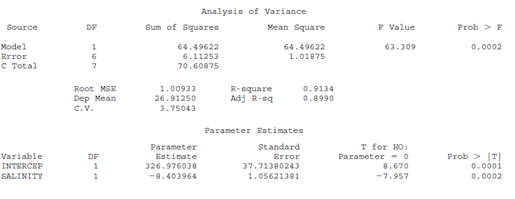
SAS output for Exercise 72
Dependent Variable: NITRLVL
Expert Solution & Answer
Want to see the full answer?
Check out a sample textbook solution
Students have asked these similar questions
Wrinkle recovery angle and tensile strength are the two most important characteristics for evaluating the performance of crosslinked cotton fabric. An increase in the degree of crosslinking, as determined by ester carboxyl band absorbance, improves the wrinkle
resistance of the fabric (at the expense of reducing mechanical strength). The accompanying data on x = absorbance and y = wrinkle resistance angle was read from a graph in the paper "Predicting the Performance of Durable Press Finished Cotton Fabric with
Infrared Spectroscopy".†
x 0.115 0.126 0.183 0.246 0.282 0.344 0.355 0.452 0.491 0.554 0.651
y 334 342 355 363
365 372 381 392
400 412 420
Here is regression output from Minitab:
Predictor
Constant
absorb
S = 3.60498
Coef
321.878
156.711
SOURCE
Regression
Residual Error
Total
SE Coef
2.483
6.464
R-Sq = 98.5%
DF
1
9
10
SS
7639.0
117.0
7756.0
T
129.64
24.24
0.000
0.000
R-Sq (adj) = 98.3%
MS
7639.0
13.0
F
P
587.81
(a) Does the simple linear regression model appear to be…
Wrinkle recovery angle and tensile strength are the two most important characteristics for evaluating the performance of crosslinked cotton fabric. An increase in the degree of crosslinking, as determined by ester carboxyl band absorbance, improves the wrinkle resistance of the fabric (at the expense of reducing mechanical
strength). The accompanying data on x = absorbance and y = wrinkle resistance angle was read from a graph in the paper "Predicting the Performance of Durable Press Finished Cotton Fabric with Infrared Spectroscopy".t
半
0.115 0.126 0.183 0.246 0.282 0.344 0.355 0.452 0.491 0.554 0.651
334 342
355
363
365
372
381
392
400
412
420
Here is regression output from Minitab:
Predictor
Coef
SE Coef
P
Constant
321.878
2.483
129.64
0.000
absorb
156.711
6.464
24.24
0.000
S = 3.60498
R-Sq = 98.5%
R-Są (adj) - 98.3%
SOURCE
DF
MS
F
P
Regression
1
7639.0
7639.0
587.81
0.000
Residual Error
9
117.0
13.0
Total
10
7756.0
(a) Does the simple linear regression model appear to be…
Wrinkle recovery angle and tensile strength are the two most important characteristics for evaluating the performance of crosslinked cotton fabric. An increase in the degree of crosslinking, as
determined by ester carboxyl band absorbance, improves the wrinkle resistance of the fabric (at the expense of reducing mechanical strength). The accompanying data on x = absorbance and
y = wrinkle resistance angle was read from a graph in the paper "Predicting the Performance of Durable Press Finished Cotton Fabric with Infrared Spectroscopy".t
x 0.115 0.126 0.183 0.246 0.282 0.344 0.355 0.452 0.491 0.554 0.651
y
334 342 355
363
365 372 381
400
392
412 420
Here is regression output from Minitab:
Predictor
Constant
absorb
S = 3.60498
Coef
321.878
156.711
SOURCE
Regression
Residual Error
Total
R-Sq= 98.5%
DF
SE Coef
2.483
6.464
1
9
10
SS
7639.0
117.0
7756..0
T
129.64
24.24
P
0.000
0.000.
R-Sq (adj) 98.3%
MS
7639.0
13.0
F
587.81
(a) Does the simple linear regression model appear to be appropriate?…
Chapter 12 Solutions
WebAssign for Devore's Probability and Statistics for Engineering and the Sciences, 9th Edition [Instant Access], Single-Term
Ch. 12.1 - The efficiency ratio for a steel specimen immersed...Ch. 12.1 - The article Exhaust Emissions from Four-Stroke...Ch. 12.1 - Bivariate data often arises from the use of two...Ch. 12.1 - The accompanying data on y = ammonium...Ch. 12.1 - The article Objective Measurement of the...Ch. 12.1 - One factor in the development of tennis elbow, a...Ch. 12.1 - The article Some Field Experience in the Use of an...Ch. 12.1 - Referring to Exercise 7, suppose that the standard...Ch. 12.1 - The flow rate y (m3/min) in a device used for...Ch. 12.1 - Suppose the expected cost of a production run is...
Ch. 12.1 - Suppose that in a certain chemical process the...Ch. 12.2 - Refer back to the data in Exercise 4, in which y =...Ch. 12.2 - The accompanying data on y = ammonium...Ch. 12.2 - Refer to the lank temperature-efficiency ratio...Ch. 12.2 - Values of modulus of elasticity (MOE, the ratio of...Ch. 12.2 - The article Characterization of Highway Runoff in...Ch. 12.2 - For the past decade, rubber powder has been used...Ch. 12.2 - For the past decade, rubber powder has been used...Ch. 12.2 - The following data is representative of that...Ch. 12.2 - The bond behavior of reinforcing bars is an...Ch. 12.2 - Wrinkle recovery angle and tensile strength are...Ch. 12.2 - Calcium phosphate cement is gaining increasing...Ch. 12.2 - a. Obtain SSE for the data in Exercise 19 from the...Ch. 12.2 - The invasive diatom species Didymosphenia geminata...Ch. 12.2 - Prob. 25ECh. 12.2 - Show that the point of averages (x,y) lies on the...Ch. 12.2 - Prob. 27ECh. 12.2 - a. Consider the data in Exercise 20. Suppose that...Ch. 12.2 - Consider the following three data sets, in which...Ch. 12.3 - Reconsider the situation described in Exercise 7,...Ch. 12.3 - During oil drilling operations, components of the...Ch. 12.3 - Exercise 16 of Section 12.2 gave data on x =...Ch. 12.3 - During oil drilling operations, components of the...Ch. 12.3 - For the past decade, rubber powder has been used...Ch. 12.3 - Refer back to the data in Exercise 4, in which y =...Ch. 12.3 - Misi (airborne droplets or aerosols) is generated...Ch. 12.3 - Prob. 37ECh. 12.3 - Refer to the data on x = liberation rate and y =...Ch. 12.3 - Carry out the model utility test using the ANOVA...Ch. 12.3 - Prob. 40ECh. 12.3 - Prob. 41ECh. 12.3 - Verify that if each xi is multiplied by a positive...Ch. 12.3 - Prob. 43ECh. 12.4 - Fitting the simple linear regression model to the...Ch. 12.4 - Reconsider the filtration ratemoisture content...Ch. 12.4 - Astringency is the quality in a wine that makes...Ch. 12.4 - The simple linear regression model provides a very...Ch. 12.4 - Prob. 48ECh. 12.4 - You are told that a 95% CI for expected lead...Ch. 12.4 - Prob. 50ECh. 12.4 - Refer to Example 12.12 in which x = test track...Ch. 12.4 - Plasma etching is essential to the fine-line...Ch. 12.4 - Consider the following four intervals based on the...Ch. 12.4 - The height of a patient is useful for a variety of...Ch. 12.4 - Prob. 55ECh. 12.4 - The article Bone Density and Insertion Torque as...Ch. 12.5 - The article Behavioural Effects of Mobile...Ch. 12.5 - The Turbine Oil Oxidation Test (TOST) and the...Ch. 12.5 - Toughness and fibrousness of asparagus are major...Ch. 12.5 - Head movement evaluations are important because...Ch. 12.5 - Prob. 61ECh. 12.5 - Prob. 62ECh. 12.5 - Prob. 63ECh. 12.5 - The accompanying data on x = UV transparency index...Ch. 12.5 - Torsion during hip external rotation and extension...Ch. 12.5 - Prob. 66ECh. 12.5 - Prob. 67ECh. 12 - The appraisal of a warehouse can appear...Ch. 12 - Prob. 69SECh. 12 - Forensic scientists are often interested in making...Ch. 12 - Phenolic compounds are found in the effluents of...Ch. 12 - The SAS output at the bottom of this page is based...Ch. 12 - The presence of hard alloy carbides in high...Ch. 12 - The accompanying data was read from a scatterplot...Ch. 12 - An investigation was carried out to study the...Ch. 12 - Prob. 76SECh. 12 - Open water oil spills can wreak terrible...Ch. 12 - In Section 12.4, we presented a formula for...Ch. 12 - Show that SSE=Syy1Sxy, which gives an alternative...Ch. 12 - Suppose that x and y are positive variables and...Ch. 12 - Let sx and sy denote the sample standard...Ch. 12 - Verify that the t statistic for testing H0: 1 = 0...Ch. 12 - Use the formula for computing SSE to verify that...Ch. 12 - In biofiltration of wastewater, air discharged...Ch. 12 - Normal hatchery processes in aquaculture...Ch. 12 - Prob. 86SECh. 12 - Prob. 87SE
Knowledge Booster


Learn more about
Need a deep-dive on the concept behind this application? Look no further. Learn more about this topic, statistics and related others by exploring similar questions and additional content below.Similar questions
- In an experiment to determine factors related to weld toughness, the Charpy V-notch impact toughness in ft - 1b (v) was measured for 22 welds at 0°Č, along with the lateral expansion at the notch in % (x,), and the brittle fracture surface in % (x2). The data are presented in the following table. X1 X2 y 32 20.0 28 39 23.0 28 20 12.8 32 21 16.0 29 25 10.2 31 20 11.6 28 32 17.6 25 29 17.8 28 27 16.0 29 43 26.2 27 22 9.6 32 22 15.2 32 18 8.8 43 32 20.4 24 22 12.2 36 25 14.6 36 25 10.4 29 20 11.6 30 20 12.6 31 24 16.2 36 18 9.2 34 28 16.8 30 a. Fit the model y = Bo + B1 X1 + ɛ. For each coefficient, test the null hypothesis that it is equal to 0. b. Fit the model y = Bo + B, xz + ɛ. For each coefficient, test the null hypothesis that it is equal to 0. c. Fit the model y = Bo + B1 X1 + Bzx2 + ɛ. For each coefficient, test the null hypothesis that it is equal to 0. d. Which of the models in parts (a) through (c) is the best of the three? Why do you think %3D + E. so?arrow_forwardGiven the “data” determined by y = x^3 + (x-1)^2 with x = 0.1, 1.2, 2.3, and 2.9, calculate SSTO, SSR, and R^2. Then recalculate these using x = 0.3, 1, 2.45, and 2.8. Does where you collect your data (i.e., which values of x) appear to impact your interpretation of how good the linear model fits?.arrow_forward17.7 Butterfly wings. Researchers studied the morphological attributes of monarch butterflies (Danaus plexippus), a species that undertakes large seasonal migrations over North America. They measured the forewing weight (in milligrams, mg) of a sample of 92 monarch butterflies, all of which had been reared in captivity in identical conditions.° Figure 17.4 shows the output from the statistical software JMP. (The data are also available in the Large.Butterfly the data file if you wish to practice working with your own software.) Estimate with 95% confidence the mean forewing weight of monarch butterflies reared in captivity. Follow the four- step process as illustrated in Example 17.2. 4 STEP そMP FWweight 30 25 20 15 10 11 12 13 14 15 8 9 10 Summary Statistics Mean 11.795652 Std Dev 1.1759413 Std Err Mean 0.1226004 Upper 95% Mean Lower 95% Mean 1 FIGURE 17.4 Software output (JMP) for the forewing weight of monarch 12.039183 11.552122 92 N. butterflies. Countarrow_forward
- Japan's high population density has resulted in a multitude of resource-usage problems. One especially serious difficulty concerns waste removal. The article "Innovative Sludge Handling Through Pelletization Thickening"t reported the development of a new compression machine for processing sewage sludge. An important part of the investigation involved relating the moisture content of compressed pellets (y, in %) to the machine's filtration rate (x, in kg-DS/m/hr). Consider the following data. 125.4 98.3 201.6 147.2 146.0 124.5 112.3 120.2 161.1 178.8 y 77.9 76.9 81.3 80.0 78.1 78.5 77.4 77.2 79.9 80.4 159.4 145.7 74.9 151.5 144.2 124.8 198.6 132.6 159.6 110.7 79.7 79.2 76.9 78.1 79.6 78.3 81.7 76.8 79.1 78.5 Relevant summary quantities are X; = 2817.4 Fy, = 1575.5, 5x? = 415,815.84, Fxy, = 222,698.08, Fy? = 124,149.53. Also, x = 140.870, y = 78.78, Sy = 18,928.7020, Sy = 757.395, and SSE = 9.222. The estimated standard deviation is o = 0.716 and the equation of the least squares line is…arrow_forwardThe following scatterplot shows the mean annual carbon dioxide (CO,) in parts (CO2) per million (ppm) measured at the top of a mountain and the mean annual air temperature over both land and sea across the globe, in degrees Celsius (C). Complete parts a through h on the right. f) View the accompanying scatterplot of the residuals vs. CO2. Does the scatterplot of the residuals vs. CO, show evidence of the violation of any assumptions behind the regression? 16.800 A. Yes, the outlier condition is violated. 16.725 O B. Yes, the linearity and equal variance assumptions are violated. 16.650 C. Yes, the equal variance assumption is violated. 16.575 O D. No, all assumptioris are okay. 16.500 O E. Yes, all the assumptions are violated. 325.0 337.5 350.0 362.5 CO2 (ppm) OF Yes, the linearity assumption is violated. his vear, What mean temperature doesarrow_forwardAn experiment to compare the tension bond strength of polymer latex modified mortar (Portland cement mortar to which polymer latex emulsions have been added during mixing) to that of unmodified mortar resulted in x = 18.11 kgf/cm² for the modified mortar (m = 42) and y = 16.82 kgf/cm² for the unmodified mortar (n = 30). Let μ₁ and μ₂ be the true average tension bond strengths for the modified and unmodified mortars, respectively. Assume that the bond strength distributions are both normal. (a) Assuming that ₁ = 1.6 and ₂ = 1.3, test Ho: ₁ - ₂ = 0 versus H₂ : ₁ - ₂ > 0 at level 0.01. Calculate the test statistic and determine the P-value. (Round your test statistic to two decimal places and your P-value to four decimal places.) z = P-value = State the conclusion in the problem context. O Reject Ho. The data does not suggest that the difference in average tension bond strengths exceeds 0. O Fail to reject Ho. The data does not suggest that the difference in average tension bond strengths…arrow_forward
- An experiment to compare the tension bond strength of polymer latex modified mortar (Portland cement mortar to which polymer latex emulsions have been added during mixing) to that of unmodified mortar resulted in x = 18.11 kgf/cm² for the modified mortar (m = 42) and y = 16.82 kgf/cm² for the unmodified mortar (n = 32). Let μ₁ and μ₂ be the true average tension bond strengths for the modified and unmodified mortars, respectively. Assume that the bond strength distributions are both normal. (a) Assuming that 0₁ = 1.6 and ₂ = 1.3, test Ho: ₁ - ₂ = 0 versus H₂: M₁-M₂ > 0 at level 0.01. Calculate the test statistic and determine the P-value. (Round your test statistic to two decimal places and your P-value to four decimal places.) z = P-value = State the conclusion in the problem context. O Reject Ho. The data does not suggest that the difference in average tension bond strengths exceeds 0. O Fail to reject Ho. The data suggests that the difference in average tension bond strengths exceeds…arrow_forward5.25. Representative data on x = carbonation depth (in millimeters) and y = strength (in megapascals) for a sample of concrete core specimens taken from a particular building were read from a plot in the article “The Carbonation of Concrete Structures in the Tropical Environment of Singapore” (Magazine of Concrete Research [1996]: 293-300): Depth, x 8.0 20.0 20.0 30.0 35.0 40.0 50.0 55.0 65.0 Strength, y 22.8 17.1 21.1 16.1 13.4 12.4 11.4 9.7 6.8 a. Construct a scatterplot. Does the relationship between carbonation depth and strength appear to be linear? Yes, the relationship between carbonation depth and strength appears to be linear however it is a negative linear relation. b. Find the equation of the of the least-squares line.c. What would you predict for strength when carbonation depth is 25 mm?d. Explain why it would not be reasonable to use the least-squares line to predict strength when carbonation depth…arrow_forwardQ3) An experiment was carried out to investigate variation of solubility of chemical X in water. The quantities in kg that dissolved in 1 liter at various temperatures are show in the table (1). Table (1) Temperature C Mass of X 2.1 2.6 2.9 3.3 15 20 25 30 35 4 50 5.1 70 7 Use the proper methods to answer the following questions: a) Draw a scatter diagram to show the data. b) Estimate the temperature based on the mass of X. c) What quantity might be expected to dissolve at 42 C? Find the quantity that your cquation indicates would dissolve at 10 C and comment on your answer.arrow_forward
- An experiment to compare the tension bond strength of polymer latex modified mortar (Portland cement mortar to which polymer latex emulsions have been added during mixing) to that of unmodified mortar resulted in x = 18.18 kgf/cm2 for the modified mortar (m = 42) and y = 16.86 kgf/cm for the unmodified mortar (n = 30). Let µ1 and Hz be the true average tension bond strengths for the modified and unmodified mortars, respectively. Assume that the bond strength distributions are both normal. (a) Assuming that o1 = 1.6 and o2 = 1.3, test Ho: µ1 - 42 = 0 versus H3: µ1 – 42 > 0 at level 0.01. Calculate the test statistic and determine the P-value. (Round your test statistic to two decimal places and your P-value to four decimal places.) z = P-value = State the conclusion in the problem context. Fail to reject Ho: The data does not suggest that the difference in average tension bond strengths exceeds from 0. o Reject Ho: The data does not suggest that the difference in average tension bond…arrow_forwardA paper gives data on x = change in Body Mass Index (BMI, in kilograms/meter2) and y = change in a measure of depression for patients suffering from depression who participated in a pulmonary rehabilitation program. The table below contains a subset of the data given in the paper and are approximate values read from a scatterplot in the paper. BMI Change (kg/m²) 0.5 -0.5 0 0.1 0.7 0.8 1 1.5 1.2 1 0.4 0.4 Depression Score Change -1 9 4 4 5 8 13 14 17 18 12 14 The accompanying computer output is from Minitab. Fitted Line Plot Depression score change = 6.512 + 5.472 BMI change 20 S 5.26270 R-Sq 27.16% R-Sq (adj) 19.88% 15- : 10- -0.5 0.0 1.5 Ⓡ S 5.26270 Coefficients Term Coef VIF SE Coef 2.26 T-Value 2.88 P-Value 0.0164 Constant 6.512 BMI change 5.472 2.83 1.93 0.0823 1.00 Regression Equation Depression score change = 6.512 + 5.472 BMI change (a) What percentage of observed variation in depression score change can be explained by the simple linear regression model? (Round your answer to…arrow_forwardA statistical program is recommended. Electromagnetic technologies offer effective nondestructive sensing techniques for determining characteristics of pavement. The propagation of electromagnetic waves through the material depends on its dielectric properties. The following data, kindly provided by the authors of the article "Dielectric Modeling of Asphalt Mixtures and Relationship with Density,"† was used to relate y = dielectric constant to x = air void (%) for 18 samples having 5% asphalt content. y 4.55 4.49 4.50 4.47 4.47 4.45 4.40 4.34 4.43 4.43 4.42 4.40 4.33 4.44 4.40 4.26 4.32 4.34 x 4.35 4.79 5.57 5.20 5.07 5.79 5.36 6.40 5.66 5.90 6.49 5.70 6.49 6.37 6.51 7.88 6.74 7.08 The following R output is from a simple linear regression of y on x. Estimate Std. Error t value Pr(>|t|) (Intercept) 4.858691 0.059768 81.283 <2e-16 AirVoid −0.074676 0.009923 −7.526 1.21e-06 Residual standard error: 0.03551 on 16 DF Multiple R-squared: 0.7797, Adjusted…arrow_forward
arrow_back_ios
SEE MORE QUESTIONS
arrow_forward_ios
Recommended textbooks for you
 MATLAB: An Introduction with ApplicationsStatisticsISBN:9781119256830Author:Amos GilatPublisher:John Wiley & Sons Inc
 Probability and Statistics for Engineering and th...StatisticsISBN:9781305251809Author:Jay L. DevorePublisher:Cengage Learning
 Statistics for The Behavioral Sciences (MindTap C...StatisticsISBN:9781305504912Author:Frederick J Gravetter, Larry B. WallnauPublisher:Cengage Learning
 Elementary Statistics: Picturing the World (7th E...StatisticsISBN:9780134683416Author:Ron Larson, Betsy FarberPublisher:PEARSON
 The Basic Practice of StatisticsStatisticsISBN:9781319042578Author:David S. Moore, William I. Notz, Michael A. FlignerPublisher:W. H. Freeman
 Introduction to the Practice of StatisticsStatisticsISBN:9781319013387Author:David S. Moore, George P. McCabe, Bruce A. CraigPublisher:W. H. Freeman
MATLAB: An Introduction with Applications
Statistics
ISBN:9781119256830
Author:Amos Gilat
Publisher:John Wiley & Sons Inc
Probability and Statistics for Engineering and th...
Statistics
ISBN:9781305251809
Author:Jay L. Devore
Publisher:Cengage Learning
Statistics for The Behavioral Sciences (MindTap C...
Statistics
ISBN:9781305504912
Author:Frederick J Gravetter, Larry B. Wallnau
Publisher:Cengage Learning
Elementary Statistics: Picturing the World (7th E...
Statistics
ISBN:9780134683416
Author:Ron Larson, Betsy Farber
Publisher:PEARSON
The Basic Practice of Statistics
Statistics
ISBN:9781319042578
Author:David S. Moore, William I. Notz, Michael A. Fligner
Publisher:W. H. Freeman
Introduction to the Practice of Statistics
Statistics
ISBN:9781319013387
Author:David S. Moore, George P. McCabe, Bruce A. Craig
Publisher:W. H. Freeman
Correlation Vs Regression: Difference Between them with definition & Comparison Chart; Author: Key Differences;https://www.youtube.com/watch?v=Ou2QGSJVd0U;License: Standard YouTube License, CC-BY
Correlation and Regression: Concepts with Illustrative examples; Author: LEARN & APPLY : Lean and Six Sigma;https://www.youtube.com/watch?v=xTpHD5WLuoA;License: Standard YouTube License, CC-BY