Essentials of Statistics (6th Edition)
6th Edition
ISBN: 9780134687155
Author: Triola
Publisher: PEARSON
expand_more
expand_more
format_list_bulleted
Concept explainers
Videos
Textbook Question
Chapter 10.2, Problem 15BSC
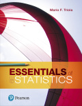
Regression and Predictions. Exercises 13–28 use the same data sets as Exercises 13–28 in Section 10-1. In each case, find the regression equation, letting the .first variable be the predictor (x) variable, Find the indicated predicted value by following the prediction procedure summarized in Figure 10-5 on page 493.
15. Pizza and the Subway Use the pizza costs and subway fares to find the best predicted subway fare, given that the cost of a slice of pizza is $3.00. Is the best predicted subway fare likely to be implemented?
Expert Solution & Answer
Want to see the full answer?
Check out a sample textbook solution
Students have asked these similar questions
Regression and Predictions. Exercises 13–28 use the same data sets as Exercises 13–28 in Section 10-1. In each case, find the regression equation, letting the first variable be the predictor (x) variable. Find the indicated predicted value by following the prediction procedure summarized in Figure 10-5 on page 493.
Tips Using the bill/tip data, find the best predicted tip amount for a dinner bill of $100. What tipping rule does the regression equation suggest?
Sam Jones has 2 years of historical sales data for his company. He is applyingfor a business loan and must supply his projections of sales by month for thenext 2 years to the bank.
a. Using the data from Table 6–12, provide a regression forecast for timeperiods 25 through 48.b. Does Sam’s sales data show a seasonal pattern?
The table gives the average heights of children for ages 1 – 10, where x = the age (in years) and y = the height (in cm). Part a: Make a scatter plot and determine which type of model best fits the data.Part b: Find the regression equation.Part c: Can your equation be used to find the average height of a 20 year old? Explain.
Chapter 10 Solutions
Essentials of Statistics (6th Edition)
Ch. 10.1 - Notation Twenty different statistics students are...Ch. 10.1 - Interpreting r For the some two variables...Ch. 10.1 - Global Warming If we find that there is a linear...Ch. 10.1 - Scatterplots Match these values of r with the five...Ch. 10.1 - Bear Weight and Chest Size Fifty-four wild bears...Ch. 10.1 - Casino Size and Revenue The New York Times...Ch. 10.1 - Garbage Data Set 31 Garbage Weight in Appendix B...Ch. 10.1 - Cereal Killers The amounts of sugar (grams of...Ch. 10.1 - Explore! Exercises 9 and 10 provide two data sets...Ch. 10.1 - Explore! Exercises 9 and 10 provide two data sets...
Ch. 10.1 - Outlier Refer to the accompanying...Ch. 10.1 - Clusters Refer to the following Minitab-generated...Ch. 10.1 - Testing for a Linear Correlation. In Exercises...Ch. 10.1 - Testing for a Linear Correlation. In Exercises...Ch. 10.1 - Testing for a Linear Correlation. In Exercises...Ch. 10.1 - Testing for a Linear Correlation. In Exercises...Ch. 10.1 - Testing for a Linear Correlation. In Exercises...Ch. 10.1 - Testing for a Linear Correlation. In Exercises...Ch. 10.1 - Testing for a Linear Correlation. In Exercises...Ch. 10.1 - Testing for a Linear Correlation. In Exercises...Ch. 10.1 - Testing for a Linear Correlation. In Exercises...Ch. 10.1 - Testing for a Linear Correlation. In Exercises...Ch. 10.1 - Testing for a Linear Correlation. In Exercises...Ch. 10.1 - Testing for a Linear Correlation. In Exercises...Ch. 10.1 - Testing for a Linear Correlation. In Exercises...Ch. 10.1 - Testing for a Linear Correlation. In Exercises...Ch. 10.1 - Testing for a Linear Correlation. In Exercises...Ch. 10.1 - Testing for a Linear Correlation. In Exercises...Ch. 10.1 - Transformed Data In addition to testing for a...Ch. 10.1 - Finding Critical r Values Table A-6 lists critical...Ch. 10.2 - Notation Different hotels on Las Vegas Boulevard...Ch. 10.2 - Notation What is the difference between the...Ch. 10.2 - Best-Fit Line a. What is a residual? b. In what...Ch. 10.2 - Correlation and Slope What is the relationship...Ch. 10.2 - Making Predictions. In Exercises 58, let the...Ch. 10.2 - Making Predictions. In Exercises 58, let the...Ch. 10.2 - Making Predictions. In Exercises 58, let the...Ch. 10.2 - Making Predictions. In Exercises 58, let the...Ch. 10.2 - Finding the Equation of the Regression Line. In...Ch. 10.2 - Finding the Equation of the Regression Line. In...Ch. 10.2 - Effects of an Outlier Refer to the Mini...Ch. 10.2 - Effects of Clusters Refer to the Minitab-generated...Ch. 10.2 - Regression and Predictions. Exercises 1328 use the...Ch. 10.2 - Regression and Predictions. Exercises 1328 use the...Ch. 10.2 - Regression and Predictions. Exercises 1328 use the...Ch. 10.2 - Regression and Predictions. Exercises 1328 use the...Ch. 10.2 - Regression and Predictions. Exercises 1328 use the...Ch. 10.2 - Regression and Predictions. Exercises 1328 use the...Ch. 10.2 - Regression and Predictions. Exercises 1328 use the...Ch. 10.2 - Regression and Predictions. Exercises 1328 use the...Ch. 10.2 - Regression and Predictions. Exercises 1328 use the...Ch. 10.2 - Regression and Predictions. Exercises 1328 use the...Ch. 10.2 - Regression and Predictions. Exercises 1328 use the...Ch. 10.2 - Regression and Predictions. Exercises 1328 use the...Ch. 10.2 - Regression and Predictions. Exercises 13-28 use...Ch. 10.2 - Regression and Predictions. Exercises 13-28 use...Ch. 10.2 - Regression and Predictions. Exercises 13-28 use...Ch. 10.2 - Regression and Predictions. Exercises 13-28 use...Ch. 10.2 - Least-Squares Property According to the...Ch. 10.3 - Regression If the methods of this section are used...Ch. 10.3 - Level of Measurement Which of the levels of...Ch. 10.3 - Notation What do r, rs , and ps denote? Why is the...Ch. 10.3 -
4. Efficiency The efficiency of the rank...Ch. 10.3 - In Exercises 5 and 6, use the scatterplot to find...Ch. 10.3 - In Exercises 5 and 6, use the scatterplot to find...Ch. 10.3 - Testing for Rank Correlation. In Exercises 712,...Ch. 10.3 - Prob. 8BSCCh. 10.3 - Testing for Rank Correlation. In Exercises 712,...Ch. 10.3 - Testing for Rank Correlation. In Exercises 712,...Ch. 10.3 - Prob. 11BSCCh. 10.3 - Testing for Rank Correlation. In Exercises 712,...Ch. 10.3 - Prob. 13BSCCh. 10.3 - Appendix B Data Sets. In Exercises 1316, use the...Ch. 10.3 - Appendix B Data Sets. In Exercises 1316, use the...Ch. 10.3 - Prob. 16BSCCh. 10.3 - Prob. 17BBCh. 10 - The following exercises are based on the following...Ch. 10 - The following exercises are based on the following...Ch. 10 - The following exercises are based on the following...Ch. 10 - The following exercises are based on the following...Ch. 10 - The following exercises are based on the following...Ch. 10 - The following exercises are based on the following...Ch. 10 - The following exercises are based on the following...Ch. 10 - The following exercises are based on the following...Ch. 10 - The following exercises are based on the following...Ch. 10 - Interpreting Scatterplot If the sample data were...Ch. 10 - Cigarette Tar and Nicotine The table below lists...Ch. 10 - 2. Cigarette Nicotine and Carbon Monoxide Refer to...Ch. 10 - Time and Motion In a physics experiment at Doane...Ch. 10 - Stocks and Sunspots. Listed below are annual high...Ch. 10 - Stocks and Sunspots. Listed below are annual high...Ch. 10 - Stocks and Sunspots. Listed below are annual high...Ch. 10 - Stocks and Sunspots. Listed below are annual high...Ch. 10 - Stocks and Sunspots. Listed below are annual high...Ch. 10 - Cell Phones and Driving In the authors home town...Ch. 10 - Ages of Moviegoers The table below shows the...Ch. 10 - Ages of Moviegoers Based on the data from...Ch. 10 - Speed Dating Data Set 18 Speed Dating" in Appendix...Ch. 10 - Speed Dating Data Set 18 Speed Dating" in Appendix...Ch. 10 - Speed Dating Data Set 18 Speed Dating" in Appendix...Ch. 10 - Speed Dating Data Set 18 Speed Dating in Appendix...Ch. 10 - Speed Dating Data Set 18 Speed Dating in Appendix...Ch. 10 - Critical Thinking: Is the pain medicine Duragesic...Ch. 10 - Critical Thinking: Is the pain medicine Duragesic...Ch. 10 - Critical Thinking: Is the pain medicine Duragesic...Ch. 10 - Critical Thinking: Is the pain medicine Duragesic...Ch. 10 - Critical Thinking: Is the pain medicine Duragesic...Ch. 10 - Prob. 4RE
Knowledge Booster


Learn more about
Need a deep-dive on the concept behind this application? Look no further. Learn more about this topic, statistics and related others by exploring similar questions and additional content below.Similar questions
- Applying the Concepts and SkillsIn Exercises, we repeat the information from Exercises. For each exercise here, discuss what satisfying Assumptions 1–3 for regression inferences by the variables under consideration would mean.ExercisesApplying the Concepts and SkillsIn each of Exercises,a. find the regression equation for the data points.b. graph the regression equation and the data points.c. describe the apparent relationship between the two variables under consideration.d. interpret the slope of the regression line.e. identify the predictor and response variables.f. identify outliers and potential influential observations.g. predict the values of the response variable for the specified values of the predictor variable, and interpret your results.Tax Efficiency.Tax efficiency is a measure, ranging from 0 to 100, of how much tax due to capital gains stock or mutual funds investors pay on their investments each year; the higher the tax efficiency, the lower is the tax. In the article…arrow_forwardCity Fuel Consumption: Finding the Best Multiple Regression Equation. In Exercises 9–12, refer to the accompanying table, which was obtained using the data from 21 cars listed in Data Set 20 “Car Measurements” in Appendix B. The response (y) variable is CITY (fuel consumption in mi/gal). The predictor (x) variables are WT (weight in pounds), DISP (engine displacement in liters), and HWY (highway fuel consumption in mi /gal). A Honda Civic weighs 2740 lb, it has an engine displacement of 1.8 L, and its highway fuel consumption is 36 mi/gal. What is the best predicted value of the city fuel consumption? Is that predicted value likely to be a good estimate? Is that predicted value likely to be very accurate?arrow_forwardCity Fuel Consumption: Finding the Best Multiple Regression Equation. In Exercises 9–12, refer to the accompanying table, which was obtained using the data from 21 cars listed in Data Set 20 “Car Measurements” in Appendix B. The response (y) variable is CITY (fuel consumption in mi/gal). The predictor (x) variables are WT (weight in pounds), DISP (engine displacement in liters), and HWY (highway fuel consumption in mi /gal). Which regression equation is best for predicting city fuel consumption? Why?arrow_forward
- City Fuel Consumption: Finding the Best Multiple Regression Equation. In Exercises 9–12, refer to the accompanying table, which was obtained using the data from 21 cars listed in Data Set 20 “Car Measurements” in Appendix B. The response (y) variable is CITY (fuel consumption in mi/gal). The predictor (x) variables are WT (weight in pounds), DISP (engine displacement in liters), and HWY (highway fuel consumption in mi /gal). If exactly two predictor (x) variables are to be used to predict the city fuel consumption, which two variables should be chosen? Why?arrow_forwardAppendix B Data Sets. In Exercises 13–16, refer to the indicated data set in Appendix B and use technology to obtain results. Predicting IQ Score Refer to Data Set 8 “IQ and Brain Size” in Appendix B and find the best regression equation with IQ score as the response (y) variable. Use predictor variables of brain volume and/or body weight. Why is this equation best? Based on these results, can we predict someone’s IQ score if we know their brain volume and body weight? Based on these results, does it appear that people with larger brains have higher IQ scores?arrow_forwardQ1. The table provided gives data on indexes of output per hour (X) and real compensation per hour (Y) for the business and nonfarm business sectors of the U.S. economy for 1960–2005. The base year of the indexes is 1992 = 100 and the indexes are seasonally adjusted. a. Plot Y against X for the two sectors separately. b. What is the economic theory behind the relationship between the two variables? Does the scattergram support the theory? c. Estimate the OLS regression of Y on X. Note: on the table ( 1. Output refers to real gross domestic product in the sector. 2. Wages and salaries of employees plus employers’ contributions for social insurance and private benefit plans. 3. Hourly compensation divided by the consumer price index for all urban consumers for recent quarters.) Thank you!arrow_forward
- What is the relationship between the amount of time statistics students study per week and their final exam scores? The results of the survey are shown below. Time Score 3 4 73 16 2 15 10 3 95 61 67 67 88 90 75 a. Find the correlation coefficient: r = b. The null and alternative hypotheses for correlation are: Hg: ?v = 0 H: ?v + 0 Round to 2 decimal places. The p-value is: (Round to four decimal places) c. Use a level of significance of a = 0.05 to state the conclusion of the hypothesis test in the context of the study. O There is statistically insignificant evidence to conclude that a student who spends more time studying will score higher on the final exam than a student who spends less time studying. O There is statistically significant evidence to conclude that there is a correlation between the time spent studying and the score on the final exam. Thus, the regression line is useful. O There is statistically insignificant evidence to conclude that there is a correlation between the…arrow_forwardA The least-squares regression equation is y = 720.8x + 14,490 where y is the median income and x is the percentage of 25 years and older with at least a bachelor's degree in the region. The scatter diagram indicates a linear relation between the two variables with a correlation coefficient of 0.7743. Complete parts (a) through (d). (a) Predict the median income of a region in which 20% of adults 25 years and older have at least a bachelor's degree. (Round to the nearest dollar as needed.) G Median Income 55000- 20000+ 15 20 25 30 35 40 45 50 55 60 Bachelor's % Qarrow_forwardPart I. Run two regressions in Excel using the provided Excel file “Layoffs”.The Excel file Layoffs provides data on 50 manufacturing workers who lost their jobs due to layoffs. The data includes the following list of variables:Weeks – the number of weeks a manufacturing worker has been without a jobAge – the age of the workerEducation – the number of years of education of the workerMarried – a dummy variable, equal to 1 if the worker is married, 0 otherwiseHead – a dummy variable, equal to 1 if the worker is a head of household, 0 otherwiseTenure – the number of years on the previous jobManager – a dummy variable, equal to 1 if the worker had a management occupation, 0 otherwise Sales – a dummy variable, equal to 1 if the worker had an occupation in sales, 0 otherwise 1. Run a simple regression with a dependent variable Weeks and an independent variable Age. Create the regular and standardized residual plots for the simple regression. 2. Run a multiple regression with a dependent…arrow_forward
- A scientist wants to develop a model to describe the relationship between the average daily temperature, x °C, and her household’s daily energy consumption, y kWh, in winter. A random sample of the average daily temperature and her household’s daily energy consumption are taken from 10 winter days and shown in the table. x -0.4 -0.2 0.3 0.8 1.1 1.4 1.8 2.1 2.5 2.6 y 28 30 26 25 26 27 26 24 22 21 You may use: Sy=255 Sxy=283.8 Syy= 64.5 Find a value for the product moment correlation coefficient r for this data Explain what the value of the product moment corelation tells you about the relationship between daily temperature and the household energy consumption.arrow_forward3. Regression analysis breaks scores on the DV into... (explain and give equations)arrow_forwardUse the data to develop a regression equationthat could be used to predict the quantity of pork sold during future periods. Discuss how you can tell whether heteroscedasticity, autocorrelation, or multi-collinearity might be a problem.arrow_forward
arrow_back_ios
SEE MORE QUESTIONS
arrow_forward_ios
Recommended textbooks for you
 Algebra & Trigonometry with Analytic GeometryAlgebraISBN:9781133382119Author:SwokowskiPublisher:Cengage
Algebra & Trigonometry with Analytic Geometry
Algebra
ISBN:9781133382119
Author:Swokowski
Publisher:Cengage
Correlation Vs Regression: Difference Between them with definition & Comparison Chart; Author: Key Differences;https://www.youtube.com/watch?v=Ou2QGSJVd0U;License: Standard YouTube License, CC-BY
Correlation and Regression: Concepts with Illustrative examples; Author: LEARN & APPLY : Lean and Six Sigma;https://www.youtube.com/watch?v=xTpHD5WLuoA;License: Standard YouTube License, CC-BY