
MATLAB: An Introduction with Applications
6th Edition
ISBN: 9781119256830
Author: Amos Gilat
Publisher: John Wiley & Sons Inc
expand_more
expand_more
format_list_bulleted
Related questions
Question
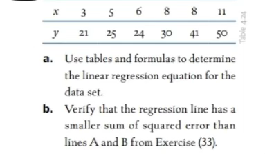

Transcribed Image Text:**Table 4.24**
| \( x \) | 3 | 5 | 6 | 8 | 11 |
|--------|---|---|---|---|----|
| \( y \) | 21 | 25 | 24 | 30 | 41 |
### Problem Statement
**a.** Use tables and formulas to determine the linear regression equation for the data set.
**b.** Verify that the regression line has a smaller sum of squared error than lines A and B from Exercise (33).

Transcribed Image Text:### Data from Exercise #33
#### Table Data
| Line A: y = 6 + 4x | Line B: y = 7 + 3.5x |
|---------------------|---------------------|
| x | 3 | 5 | 6 | 8 | 11 |
| y | 21 | 25 | 24 | 30 | 41 | 50 |
#### Scatterplot of y vs x
The scatterplot depicts the relationship between variable x and variable y. Individual data points are marked with red dots. Two linear regression lines are shown:
- **Line A**: Represented by the equation \( y = 6 + 4x \), this line is labeled as "A" on the graph.
- **Line B**: Represented by the equation \( y = 7 + 3.5x \), this line is labeled as "B" on the graph.
**Axes:**
- The x-axis ranges from 3 to 11, consistent with the values provided in the table.
- The y-axis ranges from 20 to 50, encompassing the calculated y-values from both Line A and Line B.
The scatterplot reveals how the given linear models (Line A and Line B) fit the data points:
- For Line A, the y-values for the given x-values are: 18, 26, 30, 38, and 50.
- For Line B, the y-values for the given x-values are: 17.5, 24.5, 28, 36, and 47.5.
Each dot's position reflects the corresponding y-value for each x as calculated by the specified equations, highlighting the relationship and differences between the two lines.
Expert Solution
This question has been solved!
Explore an expertly crafted, step-by-step solution for a thorough understanding of key concepts.

Step by stepSolved in 4 steps with 35 images

Knowledge Booster

Similar questions
- Show your work please.arrow_forwardAn instructor asked a random sample of eight students to record their study times at the beginning of a course. She then made a table for total hours studied (x) over 2 weeks and test score (y) at the end of the 2 weeks. The table is given below. Complete parts (a) through (f). x 10 13 10 18 6 15 16 21 y 93 79 81 74 85 81 85 80 a. Find the regression equation for the data points. b. Graph the regresson equation c. Describe the apparent relationship between the two variables. d. Identify the predictor and response variables. e. Identify outliers and potential influential observations. f.Predict the score for a student that studies for 17 hours.arrow_forwardUse the data in the table below to complete parts (a) through (d). x 37 34 40 46 42 50 62 56 51 y 22 20 25 32 27 30 30 25 28 Find the equation of the regression line. y=arrow_forward
- Use the data in the table below to complete parts (a) through (d). 39 33 40 47 42 50 59 56 51 24 22 27 32 30 31 31 27 29 Click the icon to view details on how to construct and interpret residual plots. (a) Find the equation of the regression line. (Round to three decimal places as needed.) (b) Construct a scatter plot of the data and draw the regression line. Plot the x-values on the horizontal axis and the y-values on the vertical axis. Choose the correct graph below. OA. В. Oc. OD. 34 70, (c) Construct a residual plot. Plot the x-values on the horizontal axis and the residuals on the vertical axis. Choose the correct graph below. O A. Ов. Oc. OD. (d) Determine if there are any patterns in the residual plot and explain what they suggest about the relationship between the variables. The residual plot a pattern because the residuals about 0. This implies the regression line a good representation of the relationship between the variables.arrow_forward1. In a manufacturing process the assembly line speed (feet per minute) was thought to affect the number of defective parts found during the impaction process. To test this theory, managers devised a situation in which the same batch of parts was inspected visually at a variety of line speeds. They collected the following data. Line Speed (x) Number of Defective Parts Found (y) 20 21 20 19 40 15 30 16 60 14 40 17 Use Microsoft Excel to generate regression output for this problem and use the information in the output to answer the following questions.arrow_forwardGrades on Midterm Grades on Final79 8464 7676 8385 9170 7586 7960 7975 8781 8263 63 The following table gives the data for the grades on the midterm exam and the grades on the final exam. Determine the equation of the regression line, yˆ=b0+b1x . Round the slope and y-intercept to the nearest thousandth.arrow_forward
arrow_back_ios
arrow_forward_ios
Recommended textbooks for you
- MATLAB: An Introduction with ApplicationsStatisticsISBN:9781119256830Author:Amos GilatPublisher:John Wiley & Sons Inc
 Probability and Statistics for Engineering and th...StatisticsISBN:9781305251809Author:Jay L. DevorePublisher:Cengage Learning
 Statistics for The Behavioral Sciences (MindTap C...StatisticsISBN:9781305504912Author:Frederick J Gravetter, Larry B. WallnauPublisher:Cengage Learning
  Elementary Statistics: Picturing the World (7th E...StatisticsISBN:9780134683416Author:Ron Larson, Betsy FarberPublisher:PEARSON
 The Basic Practice of StatisticsStatisticsISBN:9781319042578Author:David S. Moore, William I. Notz, Michael A. FlignerPublisher:W. H. Freeman
 Introduction to the Practice of StatisticsStatisticsISBN:9781319013387Author:David S. Moore, George P. McCabe, Bruce A. CraigPublisher:W. H. Freeman
MATLAB: An Introduction with Applications
Statistics
ISBN:9781119256830
Author:Amos Gilat
Publisher:John Wiley & Sons Inc
Probability and Statistics for Engineering and th...
Statistics
ISBN:9781305251809
Author:Jay L. Devore
Publisher:Cengage Learning
Statistics for The Behavioral Sciences (MindTap C...
Statistics
ISBN:9781305504912
Author:Frederick J Gravetter, Larry B. Wallnau
Publisher:Cengage Learning
Elementary Statistics: Picturing the World (7th E...
Statistics
ISBN:9780134683416
Author:Ron Larson, Betsy Farber
Publisher:PEARSON
The Basic Practice of Statistics
Statistics
ISBN:9781319042578
Author:David S. Moore, William I. Notz, Michael A. Fligner
Publisher:W. H. Freeman
Introduction to the Practice of Statistics
Statistics
ISBN:9781319013387
Author:David S. Moore, George P. McCabe, Bruce A. Craig
Publisher:W. H. Freeman